2.1 What happens when we render?
R Markdown combines several different processes together to create documents, and one of the main sources of confusion from R Markdown is how all the components work together.2 Fortunately, as a user, it is not essential to understand all the inner workings of these processes to be able to create documents. However, as a user who may be seeking to alter the behavior of a document, it is important to understand which component is responsible for what. This makes it a lot easier to seek help as you can target your searches on the correct area.
The basic workflow structure for an R Markdown document is shown in Figure 2.1, highlighting the steps (arrows) and the intermediate files that are created before producing the output. The whole process is implemented via the function rmarkdown::render(). Each stage is explained in further detail below.
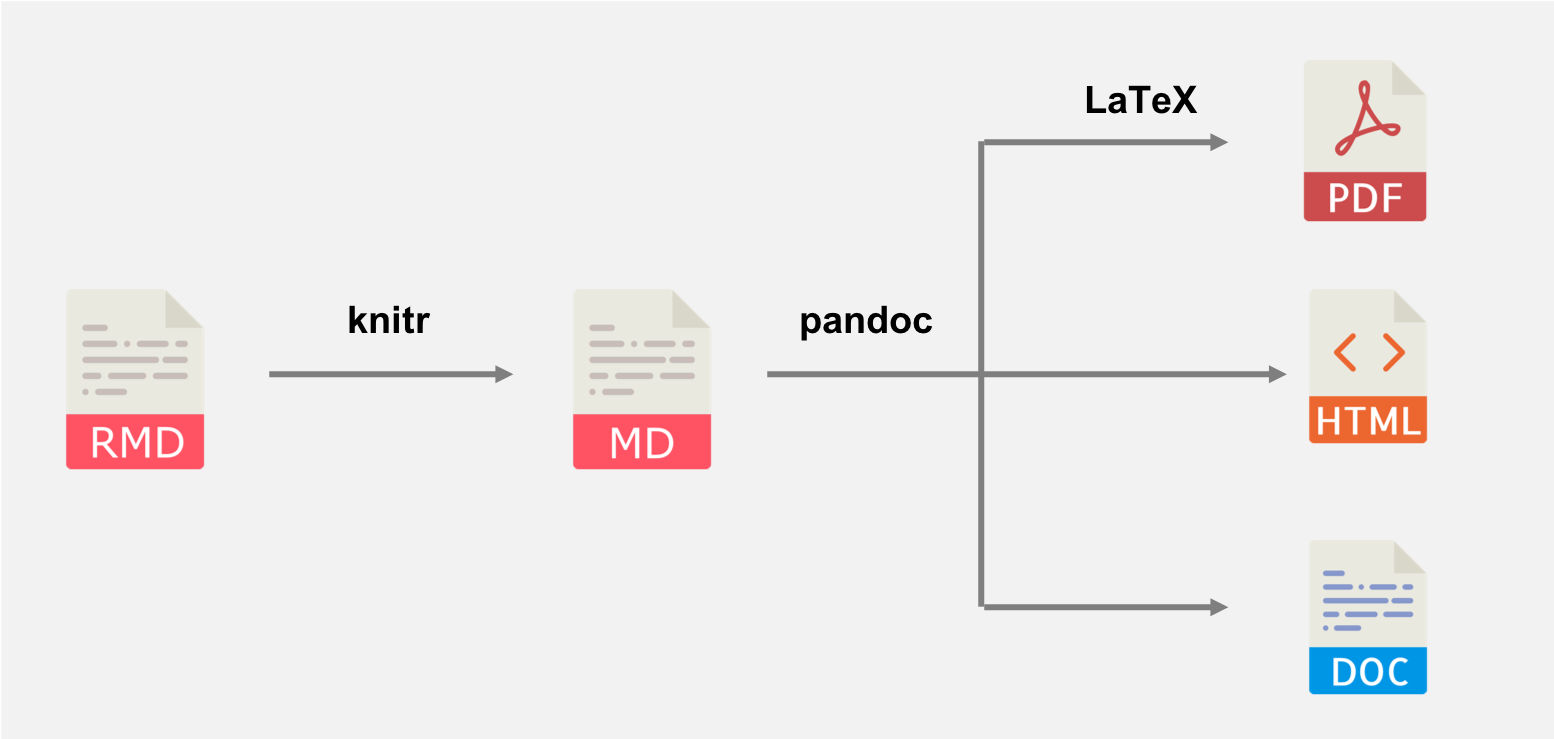
FIGURE 2.1: A diagram illustrating how an R Markdown document is converted to the final output document.
The .Rmd document is the original format of the document. It contains a combination of YAML (metadata), text (narratives), and code chunks.
First, the knit() function in knitr (Xie 2025c) is used to execute all code embedded within the .Rmd file, and prepare the code output to be displayed within the output document. All these results are converted into the correct markup language to be contained within the temporary .md file.
Then the .md file is processed by Pandoc, a multipurpose tool designed to convert files from one markup language to another. It takes any parameters specified within the YAML frontmatter of the document (e.g., title, author, and date) to convert the document to the output format specified in the output parameter (such as html_document for HTML output).
If the output format is PDF, there is an additional layer of processing, as Pandoc will convert the intermediate .md file into an intermediate .tex file. This file is then processed by LaTeX to form the final PDF document. As we mentioned in Section 1.2, the rmarkdown package calls the latexmk() function in the tinytex package (Xie 2025d), which in turn calls LaTeX to compile .tex to .pdf.
In short, rmarkdown::render() = knitr::knit() + Pandoc (+ LaTeX for PDF output only).
Robin Linacre has written a nice summary of the relationship between R Markdown, knitr, and Pandoc at https://stackoverflow.com/q/40563479/559676, which contains more technical details than the above overview.
Note that not all R Markdown documents are eventually compiled through Pandoc. The intermediate .md file could be compiled by other Markdown renderers. Below are two examples:
The xaringan package (Xie 2025e) passes the
.mdoutput to a JavaScript library, which renders the Markdown content in the web browser.The blogdown package (Xie, Dervieux, and Presmanes Hill 2025) supports the
.Rmarkdowndocument format, which is knitted to.markdown, and this Markdown document is usually rendered to HTML by an external site generator.
References
Allison Horst has created an amusing artwork that describes the R Markdown process as wizardry: https://github.com/allisonhorst/stats-illustrations/raw/master/rstats-artwork/rmarkdown_wizards.png. As a matter of fact, the cover image of this book was adapted from this artwork.↩︎