11.14 Post-process plots (*)
After a plot is generated from a code chunk, you can post-process the plot file via the chunk option fig.process, which should be a function that takes the file path as the input argument and returns a path to the processed plot file. This function can have an optional second argument options, which is a list of the current chunk options.
Below we show an example of adding an R logo to a plot using the extremely powerful magick package (Ooms 2025). If you are not familiar with this package, we recommend that you read its online documentation or package vignette, which contains lots of examples. First, we define a function add_logo():
add_logo <- function(path, options) {
  # the plot created from the code chunk
  img <- magick::image_read(path)
  # the R logo
  logo <- file.path(R.home("doc"), "html", "logo.jpg")
  logo <- magick::image_read(logo)
  # the default gravity is northwest, and users can
  # change it via the chunk option magick.gravity
  if (is.null(g <- options$magick.gravity))
    g <- "northwest"
  # add the logo to the plot
  img <- magick::image_composite(img, logo, gravity = g)
  # write out the new image
  magick::image_write(img, path)
  path
}
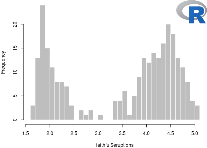
Basically the function takes the path of an R plot, adds an R logo to it, and saves the new plot to the original path. By default, the logo is added to the upper-left corner (northwest) of the plot, but users can customize the location via the custom chunk option magick.gravity (this option name can be arbitrary).
Now we apply the above processing function to the code chunk below with chunk options fig.process = add_logo and magick.gravity = "northeast", so the logo is added to the upper-right corner. See Figure 11.1 for the actual output.
par(mar = c(4, 4, 0.1, 0.1))
hist(faithful$eruptions, breaks = 30, main = "", col = "gray",
  border = "white")
FIGURE 11.1: Add the R logo to a plot via the chunk option fig.process.
After you get more familiar with the magick package, you may come up with more creative and useful ideas to post-process your R plots.
Finally, we show one more application of the fig.process option. The pdf2png() function below converts a PDF image to PNG. In Section 11.15, we have an example of using the tikz graphical device to generate plots. The problem is that this device generates PDF plots, which will not work for non-LaTeX output documents. With the chunk options dev = "tikz" and fig.process = pdf2png, we can show the PNG version of the plot in Figure 11.2.
pdf2png <- function(path) {
  # only do the conversion for non-LaTeX output
  if (knitr::is_latex_output())
    return(path)
  path2 <- xfun::with_ext(path, "png")
  img <- magick::image_read_pdf(path)
  magick::image_write(img, path2, format = "png")
  path2
}