17 논리형과 수치형
17.1 들어가기
이 장에서는 논리형과 수치형 벡터를 다루는 편리한 도구들을 배울 것입니다.
이 두 타잎은 다음과 같은 중요한 연결점이 있기 때문에 함께 배울 것입니다: 수치형 문맥에서 논리형 벡터를 사용하면 TRUE 는 1, FALSE 는 0 이 되고, 논리형 문맥에서 수치형 벡터를 사용하면, 0 은 FALSE 가, 그외 모든 것은 TRUE 가 됩니다.
17.2 논리형 벡터
논리형 벡터의 요소가 가질 수 있는 값은 세 가지 입니다: TRUE, FALSE, NA.
17.2.1 불리안 연산
filter() 에서 다중 조건을 사용하면, 모든 조건이 TRUE 인 행만 반환됩니다.
R 에서 & 는 논리형 “and” 를 의미하기 때문에, df %>% filter(cond1, cond2) 는 df %>% filter(cond1 & cond2) 와 같습니다.
다른 종류의 조합에 대해서, 직접 불리안 연산을 사용해야 합니다: | 는 “or”, ! 는 “not” 입니다.
Figure 17.1 에 불리안 연산 전체 목록이 있습니다.
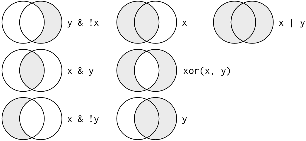
Figure 17.1: Complete set of boolean operations. x is the left-hand circle, y is the right-hand circle, and the shaded region show which parts each operator selects."
다음 코드는 11월과 12월에 출발한 모든 항공편을 불러옵니다.
연산 순서가 영어와 같게 되지 않는 것을 주목할 수 있습니다.
filter(flights, month == 11 | 12) 라고 쓰면 “find all flights that departed in November or December” 라고 읽을 수 있겠지만, 이렇게 작성하면 안됩니다.
사실 이렇게 하면 더 복잡하게 됩니다.
우선 11 | 12 을 evaluate 하는데 이는 TRUE | TRUE 와 같기 때문에 최종적으로 TRUE 를 반환합니다.
그리고 나서 month == TRUE 라고 evaluate 합니다.
month 가 수치형이기 때문에, 이는 month == 1 와 같아지기 때문에 이 표현은 1월의 모든 항공편을 불러오게 됩니다!
이 문제를 가장 쉽게 푸는 방법은 %in% 을 사용하는 것입니다.
x %in% y 를 하면 x 의 값이 y 중 어느 곳에 포함될 때마다 TRUE 인, x 와 같은 길이의 논리형 벡터를 반환합니다.
따라서 위 코드를 다시 작성하기 위해 사용할 수 있습니다:
드 모르간의 법칙을 사용하여 복잡한 서브셋하기를 단순화 할 수도 있다:
!(x & y) 는 !x | !y 와 같고, !(x | y) 는 !x & !y 와 같다.
예를 들어, 두 시간 이상 연기되지 않은 (도착이나 출발에 있어) 항공편을 모두 불러오고 싶으면, 다음 두 필터 중 하나를 사용하면 됩니다:
flights %>% filter(!(arr_delay > 120 | dep_delay > 120))
flights %>% filter(arr_delay <= 120, dep_delay <= 120)
R 에는 & 와 | 뿐만 아니라, && 와 || 도 있습니다.
dplyr 함수에서는 이 두 연산자를 사용하지 마세요!
이들은 short-circuiting 연산자라고 불리는데 조건부 실행에 관한 ?? 장에서 이들을 사용할 때 배우게 될 것입니다.
17.2.2 결측값
filter() 를 하면 논리형 표현식이 TRUE 인 행만 선택됩니다; 결측이거나 FALSE 인 행은 선택되지 않습니다.
결측값을 포함한 행을 선택하고 싶으면, in.na() 를 사용하여 결측을 논리형 벡터로 변환해야 합니다.
flights %>% filter(is.na(dep_delay) | is.na(arr_delay))
#> # A tibble: 9,430 × 19
#>    year month   day dep_time sched_dep_time dep_delay arr_time sched_arr_time
#>   <int> <int> <int>    <int>          <int>     <dbl>    <int>          <int>
#> 1  2013     1     1     1525           1530        -5     1934           1805
#> 2  2013     1     1     1528           1459        29     2002           1647
#> 3  2013     1     1     1740           1745        -5     2158           2020
#> 4  2013     1     1     1807           1738        29     2251           2103
#> 5  2013     1     1     1939           1840        59       29           2151
#> 6  2013     1     1     1952           1930        22     2358           2207
#> # … with 9,424 more rows, and 11 more variables: arr_delay <dbl>,
#> #   carrier <chr>, flight <int>, tailnum <chr>, origin <chr>, dest <chr>,
#> #   air_time <dbl>, distance <dbl>, hour <dbl>, minute <dbl>, time_hour <dttm>
flights %>% filter(is.na(dep_delay) != is.na(arr_delay))
#> # A tibble: 1,175 × 19
#>    year month   day dep_time sched_dep_time dep_delay arr_time sched_arr_time
#>   <int> <int> <int>    <int>          <int>     <dbl>    <int>          <int>
#> 1  2013     1     1     1525           1530        -5     1934           1805
#> 2  2013     1     1     1528           1459        29     2002           1647
#> 3  2013     1     1     1740           1745        -5     2158           2020
#> 4  2013     1     1     1807           1738        29     2251           2103
#> 5  2013     1     1     1939           1840        59       29           2151
#> 6  2013     1     1     1952           1930        22     2358           2207
#> # … with 1,169 more rows, and 11 more variables: arr_delay <dbl>,
#> #   carrier <chr>, flight <int>, tailnum <chr>, origin <chr>, dest <chr>,
#> #   air_time <dbl>, distance <dbl>, hour <dbl>, minute <dbl>, time_hour <dttm>
17.2.3 mutate() 에서
filter() 에서 복잡하고 여러부분으로 된 표현식을 사용하기 시작할 때마다, 명시적인 변수들을 대신 만드는 것을 고려하십시오.
이렇게 하면 작업을 확인하기 훨씬 쉬워집니다.
당신의 작업을 확인할때, mutate() 인수 중 특별히 유용한 것은 .keep = "used: 입니다: 생성한 변수와 함께 사용한 변수들이 보여질 것입니다.
연관된 변수들을 쉽게 바로 옆에 볼 수 있게 됩니다.
flights %>%
  mutate(is_cancelled = is.na(dep_delay) | is.na(arr_delay), .keep = "used") %>%
  filter(is_cancelled)
#> # A tibble: 9,430 × 3
#>   dep_delay arr_delay is_cancelled
#>       <dbl>     <dbl> <lgl>
#> 1        -5        NA TRUE
#> 2        29        NA TRUE
#> 3        -5        NA TRUE
#> 4        29        NA TRUE
#> 5        59        NA TRUE
#> 6        22        NA TRUE
#> # … with 9,424 more rows
17.2.4 조건부 아웃풋
조건식이 참일 때 하나의 값을, FALSE 일 때 다른 값을 사용하고 싶다면, if_else()5 을 사용하면 됩니다.
df <- data.frame(
  date = as.Date("2020-01-01") + 0:6,
  balance = c(100, 50, 25, -25, -50, 30, 120)
)
df %>% mutate(status = if_else(balance < 0, "overdraft", "ok"))
#>         date balance    status
#> 1 2020-01-01     100        ok
#> 2 2020-01-02      50        ok
#> 3 2020-01-03      25        ok
#> 4 2020-01-04     -25 overdraft
#> 5 2020-01-05     -50 overdraft
#> 6 2020-01-06      30        ok
#> 7 2020-01-07     120        ok
여러 if_else 들을 중첩하여 사용하게 된다면, 이 것보다는 case_when() 을 사용하기를 제안합니다.
case_when() 은 특별한 문법을 가지고 있습니다: condition ~ output 같은 형태를 가진 쌍을 입력으로 합니다.
condition 은 논리형 벡터로 평가되어야 합니다; TRUE 일 때의, output 이 사용될 것입니다.
df %>%
  mutate(
    status = case_when(
      balance == 0 ~ "no money",
      balance  < 0 ~ "overdraft",
      balance  > 0 ~ "ok"
    )
  )
#>         date balance    status
#> 1 2020-01-01     100        ok
#> 2 2020-01-02      50        ok
#> 3 2020-01-03      25        ok
#> 4 2020-01-04     -25 overdraft
#> 5 2020-01-05     -50 overdraft
#> 6 2020-01-06      30        ok
#> 7 2020-01-07     120        ok
(나는 보통 output 라인에 공백을 추가해서 빠르게 보기 쉽게 한다) 매치된 케이스가 없다면, output 은 결측이 될 것입니다:
x <- 1:10
case_when(
  x %% 2 == 0 ~ "even",
)
#>  [1] NA     "even" NA     "even" NA     "even" NA     "even" NA     "even"
조건식에 TRUE 를 사용하여, 모든 값에 대해 캐치를 생성할 수 있습니다:
case_when(
  x %% 2 == 0 ~ "even",
  TRUE        ~ "odd"
)
#>  [1] "odd"  "even" "odd"  "even" "odd"  "even" "odd"  "even" "odd"  "even"
다중 조건식이 TRUE 이면, 첫번재가 사용됩니다:
case_when(
  x < 5 ~ "< 5",
  x < 3 ~ "< 3",
)
#>  [1] "< 5" "< 5" "< 5" "< 5" NA    NA    NA    NA    NA    NA
17.2.5 요약함수
논리형 벡터에 특별히 유용한 요약 함수 네 개가 있습니다: 네 함수 모두 논리형 값 벡터를 입력으로 하고 하나의 값을 반환하기 때문에, summarize() 에서 사용하기에 알맞습니다.
any() 와 all() — any() 는 TRUE 가 적어도 하나가 있으면 TRUE 를 반환하고, all() 은 모든 값이 TRUE 이면 TRUE 를 반환합니다.
결측이 하나라도 있으면, 다른 요약함수와 같이 NA 를 반환하는데, na.rm = TRUE 를 사용하여 결측값을 제거할 수 있습니다.
sum() 와 mean() 는 논리형 벡터와 사용할 때 유용한데, TRUE 는 1 로 FALSE 는 0 으로 변환되기 때문입니다.
따라서 sum(x) 를 하면 x 에서 TRUE 의 개수를, mean(x) 을 하면 TRUE 의 비율을 얻을 수 있습니다:
not_cancelled <- flights %>% filter(!is.na(dep_delay), !is.na(arr_delay))

# How many flights left before 5am? (these usually indicate delayed
# flights from the previous day)
not_cancelled %>%
  group_by(year, month, day) %>%
  summarise(n_early = sum(dep_time < 500))
#> # A tibble: 365 × 4
#> # Groups:   year, month [12]
#>    year month   day n_early
#>   <int> <int> <int>   <int>
#> 1  2013     1     1       0
#> 2  2013     1     2       3
#> 3  2013     1     3       4
#> 4  2013     1     4       3
#> 5  2013     1     5       3
#> 6  2013     1     6       2
#> # … with 359 more rows

# What proportion of flights are delayed by more than an hour?
not_cancelled %>%
  group_by(year, month, day) %>%
  summarise(hour_prop = mean(arr_delay > 60))
#> # A tibble: 365 × 4
#> # Groups:   year, month [12]
#>    year month   day hour_prop
#>   <int> <int> <int>     <dbl>
#> 1  2013     1     1    0.0722
#> 2  2013     1     2    0.0851
#> 3  2013     1     3    0.0567
#> 4  2013     1     4    0.0396
#> 5  2013     1     5    0.0349
#> 6  2013     1     6    0.0470
#> # … with 359 more rows
17.2.6 Exercises
- For each plane, count the number of flights before the first delay of greater than 1 hour.
- What does
prod()return when applied to a logical vector? What logical summary function is it equivalent to? What doesmin()return applied to a logical vector? What logical summary function is it equivalent to?
17.3 수치형 벡터
17.3.1 변환
mutate() 로 사용할 수 있는 새로운 변수를 생성하는 함수가 많이 있습니다.
핵심 조건은 함수가 벡터화되어야 한다는 것입니다: 값들이 있는 벡터를 입력으로 하고, 같은 숫자의 값을 가진 벡터를 아웃풋으로 리턴해야 합니다.
사용할 수 있는 모든 가능한 함수를 나열하는 법은 없겠지만, 유용한 함수를 골라보았습니다:
산술 연산:
+,-,*,/,^. “재사용 법칙” 이라고 불리는 것을 사용하여 모두 벡터화됩니다. 한 파라미터가 다른 것보다 짧으면, 같은 길이까지 자동으로 연장됩니다. 한 인수가 단일 숫자일 때 매우 유용합니다:air_time / 60,hours * 60 + minute, 등.삼각함수: R 은 예상하는 삼각함수 모두가 있습니다. 데이터 과학에서 삼각함수가 필요한 경우가 많이 없기 때문에 여기서 전체 함수를 나열하지 않겠습니다. 하지만, 필요하면 사용할 수 있다는 것을 알면서 밤에 편안히 자면 됩니다.
-
모듈러 대수:
%/%(정수 나누기) 와%%(나머지), 다음이 성립:x == y * (x %/% y) + (x %% y). 모듈러 대수는 정수를 분해할 수 있게 하기 때문에 편리한 도구입니다. 예를 들어, flights 데이터셋에서,dep_time에서hour와minute을 다음과 같이 계산할 수 있습니다: -
로그:
log(),log2(),log10(). 로그는 여러 차수를 넘나드는 데이터를 처리하는 데 매우 유용한 변환입니다. 곱하기 관계를 더하기 관계로도 변환합니다.다른 조건이 같다면
log2()를 사용할 것을 추천하는데 해석이 다음과 같이 쉽기 때문입니다: 로그 스케일에서 1 차이는 원 스케일에서 두 배에 해당하고 -1 차이는 절반에 해당합니다. round(). Negative numbers.
flights %>%
  group_by(hour = sched_dep_time %/% 100) %>%
  summarise(prop_cancelled = mean(is.na(dep_time)), n = n()) %>%
  filter(hour > 1) %>%
  ggplot(aes(hour, prop_cancelled)) +
  geom_point()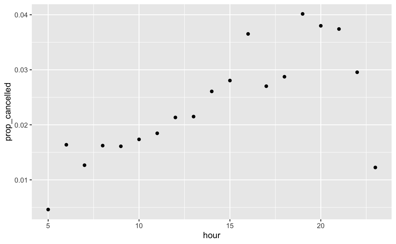
17.3.2 요약함수
mean, count, sum 을 사용하는 것만으로도 많은 이점이 있지만, R 에는 유용한 요약 함수들이 많습니다:
-
위치측정값: 앞서
mean(x)를 사용했지만,median(x)도 유용하다. 평균(mean)은 총합 나누기 길이이고 중앙값(median)은x의 50% 가 위에 위치하고, 50% 는 아래에 위치하게 되는 값이다.not_cancelled %>% group_by(month) %>% summarise( med_arr_delay = median(arr_delay), med_dep_delay = median(dep_delay) ) #> # A tibble: 12 × 3 #> month med_arr_delay med_dep_delay #> <int> <dbl> <dbl> #> 1 1 -3 -2 #> 2 2 -3 -2 #> 3 3 -6 -1 #> 4 4 -2 -2 #> 5 5 -8 -1 #> 6 6 -2 0 #> # … with 6 more rows집계와 논리형 서브셋을 조합하는 것이 유용할 때가 있다. 이러한 종류의 서브셋하기를 아직 우리가 다루지는 않았지만, 28.4.5 에서 더 배울 것이다.
not_cancelled %>% group_by(year, month, day) %>% summarise( avg_delay1 = mean(arr_delay), avg_delay2 = mean(arr_delay[arr_delay > 0]) # the average positive delay ) #> # A tibble: 365 × 5 #> # Groups: year, month [12] #> year month day avg_delay1 avg_delay2 #> <int> <int> <int> <dbl> <dbl> #> 1 2013 1 1 12.7 32.5 #> 2 2013 1 2 12.7 32.0 #> 3 2013 1 3 5.73 27.7 #> 4 2013 1 4 -1.93 28.3 #> 5 2013 1 5 -1.53 22.6 #> 6 2013 1 6 4.24 24.4 #> # … with 359 more rows -
산포측정값:
sd(x),IQR(x),mad(x). 평균제곱편차, 혹은 표준편차(standard deviation)인sd(x)는 산포의 표준측 정값이다. 사분위범위(interquartile range),IQR(x)과 중위절대편차(median absolute deviation),mad(x)는 이상값이 있을 때 더 유용하고, 로버스트한 대체 측정값들이다.# Why is distance to some destinations more variable than to others? not_cancelled %>% group_by(origin, dest) %>% summarise(distance_sd = sd(distance), n = n()) %>% filter(distance_sd > 0) #> # A tibble: 2 × 4 #> # Groups: origin [2] #> origin dest distance_sd n #> <chr> <chr> <dbl> <int> #> 1 EWR EGE 0.500 106 #> 2 JFK EGE 0.498 101 # Did it move? not_cancelled %>% filter(dest == "EGE") %>% select(time_hour, dest, distance, origin) %>% ggplot(aes(time_hour, distance, colour = origin)) + geom_point()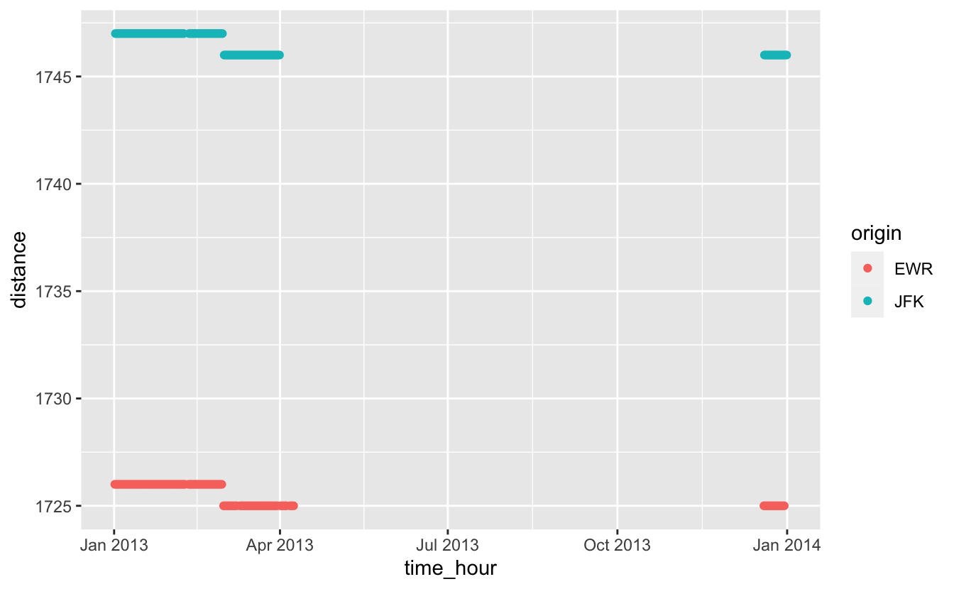
-
순위측정값:
min(x),quantile(x, 0.25),max(x). 분위수는 중앙값의 일반화이다. 예를 들어quantile(x, 0.25)는x중 25% 보다는 크고 나머지 75% 보다는 작은 값을 찾는다.# When do the first and last flights leave each day? not_cancelled %>% group_by(year, month, day) %>% summarise( first = min(dep_time), last = max(dep_time) ) #> # A tibble: 365 × 5 #> # Groups: year, month [12] #> year month day first last #> <int> <int> <int> <int> <int> #> 1 2013 1 1 517 2356 #> 2 2013 1 2 42 2354 #> 3 2013 1 3 32 2349 #> 4 2013 1 4 25 2358 #> 5 2013 1 5 14 2357 #> 6 2013 1 6 16 2355 #> # … with 359 more rows
17.3.3 mutate 에서 요약함수
mutate() 내부에서 요약함수를 사용할 때, 자동으로 올바른 길이로 재활용됩니다.
- 사칙연산은 이후에 배울 집계 함수와 함께 사용할 때 유용합니다.
예를 들어,
x / sum(x)전체에서 비율을 계산하고,y - mean(y)는 평균에서 차이를 계산합니다.
17.3.4 논리형 비교
<, <=, >, >=, !=, ==.
일련의 복잡한 논리형 연산을 하고 있다면, 새로운 변수에 중간 값을 저장하여 각 단계가 제대로 돌아가고 있는지 확인하는 것이 좋습니다.
between(x, low, high) 는 x >= low & x <= high 와 같은데, 조금 타이핑을 덜해도 되는 유용한 단축어 입니다.
닫힌 구간 (exclusive between)이나 왼쪽-열린, 오른쪽-닫힌 등을 원하면, 수작업으로 작성해야 합니다.
== 을 수치형과 사용한 결과는 예상치 못한 경우가 많으므로, 조심해야합니다!
(sqrt(2) ^ 2) == 2
#> [1] FALSE
(1 / 49 * 49) == 1
#> [1] FALSE
컴퓨터는 유한 정밀도 산술을 사용하므로 (당연히 무한개의 숫자를 저장할 수 없음!) 보이는 모든 숫자는 근사임을 기억하세요.
(sqrt(2) ^ 2) - 2
#> [1] 4.44e-16
(1 / 49 * 49) - 1
#> [1] -1.11e-16
== 대신, 적은 오차를 허용하는 near() 을 사용하세요:
다른 방법으로, round() 를 사용하여 필요없는 숫자를 잘라낼 수 있습니다.
17.4 Exercises
What trigonometric functions does R provide?
-
Brainstorm at least 5 different ways to assess the typical delay characteristics of a group of flights. Consider the following scenarios:
A flight is 15 minutes early 50% of the time, and 15 minutes late 50% of the time.
A flight is always 10 minutes late.
A flight is 30 minutes early 50% of the time, and 30 minutes late 50% of the time.
99% of the time a flight is on time. 1% of the time it’s 2 hours late.
Which is more important: arrival delay or departure delay?