5 데이터 변환

5.1 들어가기

시각화는 직관을 얻을 수 있는 중요한 도구이다. 하지만 데이터가 정확히 필요한 형태를 취하는 경우는 거의 없다. 데이터를 좀 더 쉽게 사용할 수 있도록 새로운 변수나 요약값을 만들어야 할 수도 있고, 아니면 변수 이름을 변경하거나 관측값들을 재정렬해야 되는 경우가 종종 있다. 이 장에서 이 모든 것(과 그 이상!)을 배울 것인데, dplyr 패키지와 2013년 뉴욕시 출발 항공편 데이터셋을 이용하여 데이터 변환 방법을 배워보자.

이 장의 목적은 데이터프레임을 변환하는 핵심 도구 모두를 종합적으로 살펴보는 것이다. 이러한 함수들을 뒷장에서 다시 자세히 살펴볼 것인데, 특수한 데이터 유형을 파 볼 것이다 (예: 수치형, 문자열, 날짜).

5.1.1 준비하기

이 장에서 우리는 tidyverse의 또 다른 핵심 구성요소인 dplyr 패키지를 사용하는 방법에 살펴볼 것이다. nycflights13 패키지의 데이터를 이용하여 핵심 아이디어를 배우고, ggplot2 를 이용하여 데이터를 이해해볼 것이다.

library(nycflights13)
library(tidyverse)
#> ── Attaching packages ─────────────────────────────────────── tidyverse 1.3.1 ──
#> ✓ ggplot2 3.3.5     ✓ purrr   0.3.4
#> ✓ tibble  3.1.6     ✓ dplyr   1.0.7
#> ✓ tidyr   1.1.4     ✓ stringr 1.4.0
#> ✓ readr   2.1.0     ✓ forcats 0.5.1
#> ── Conflicts ────────────────────────────────────────── tidyverse_conflicts() ──
#> x dplyr::filter() masks stats::filter()
#> x dplyr::lag()    masks stats::lag()

tidyverse 를 로드할 때 출력되는 충돌 메시지를 조심히 살펴보라. dplyr 이 베이스 R 함수 몇 개를 덮어쓴다고 알려준다. dplyr를 로딩한 후 이 함수들의 베이스 버전을 사용하고 싶다면 stats::filter(), stats::lag() 와 같이 전체 이름을 사용해야 한다.

5.1.2 nycflights13

dplyr의 기본 데이터 작업(manipulation) 동사를 탐색하기 위해서 nycflights13::flights 를 사용할 것이다. 이 데이터프레임에는 뉴욕시에서 2013년에 출발한 336,776 편의 모든 항공편이 포함되어 있다. 데이터의 출처는 Bureau of Transportation Statistics이며 ?flights 에 문서화되어 있다.

flights
#> # A tibble: 336,776 × 19
#>    year month   day dep_time sched_dep_time dep_delay arr_time sched_arr_time
#>   <int> <int> <int>    <int>          <int>     <dbl>    <int>          <int>
#> 1  2013     1     1      517            515         2      830            819
#> 2  2013     1     1      533            529         4      850            830
#> 3  2013     1     1      542            540         2      923            850
#> 4  2013     1     1      544            545        -1     1004           1022
#> 5  2013     1     1      554            600        -6      812            837
#> 6  2013     1     1      554            558        -4      740            728
#> # … with 336,770 more rows, and 11 more variables: arr_delay <dbl>,
#> #   carrier <chr>, flight <int>, tailnum <chr>, origin <chr>, dest <chr>,
#> #   air_time <dbl>, distance <dbl>, hour <dbl>, minute <dbl>, time_hour <dttm>

R 을 사용해본 독자라면 이 데이터프레임은 이전에 사용했던 데이터프레임과 조금 다르게 출력되는 것을 알아차렸을 것이다. 데이터가 티블(tibble) 이기 때문인데, tidyverse 팀에서 data.frame 의 불편한 점을 피하기 위해 고안한 특수한 종류의 데이터프레임이다. 가장 중요한 차이는 출력하는 방법에 있다. 티블은 큰 데이터셋을 위해 설계되었기 때문에 처음 몇 행과 한 화면에 들어갈 개수의 열만 표시된다. 데이터셋 전체를 보려면 View(flights) 를 실행하여 RStudio 뷰어에서 데이터셋을 열 수 있다. 다른 중요한 차이점들은 14 장에서 살펴볼 것이다.

열 이름 아래의 세 글자(또는 네 글자) 줄임말 행을 봤을 것이다. 이는 각 변수의 유형을 설명한다: <int> 는 정수형(integer)의 줄임말, <dbl> 은 더블형(double), 즉 실수의 줄임말, <chr> 은 문자형 (character, 다른말로 문자열)의 줄임말, <dttm> 은 데이트-타임형(날짜-시간)의 줄임말이다. 열에 적용하는 연산은 열 유형에 따라 달라지므로 이러한 것들은 중요하고, 이 책의 변환 섹션의 장들을 정리하는데 사용된다.

5.1.3 dplyr 기초

이 장에서는 데이터 작업 문제 대부분을 풀 수 있는 핵심 dplyr 동사들을 배울 것이다. 모든 dplyr 동사들은 비슷하게 작동한다:

1. 첫번째 인수는 데이터프레임이다.

2. 그 이후의 인수들은 (따옴표가 없는) 변수 이름을 사용하여 데이터프레임에 무엇을 할지를 설명한다.

3. 결과는 새로운 데이터프레임이다.

따라서 dplyr 코드는 다음과 같이 생기게 된다:

data |> 
  filter(x == 1) |> 
  mutate(
    y = x + 1
  )

|> 는 파이프라는 이름의 특수연산자이다. 이 연산자는 왼쪽에 있는 것을 오른쪽에 있는 함수에 전달한다. 파이프를 읽는 가장 쉬운 방법은 “그 다음” 이다. 위 코드를, 데이터를 가져와서, 그 다음 필터를 하고, 그 다음 변형을 하라 라고 읽을 수 있다. 파이프와 다른 방법을 ?? 에서 다시 살펴볼 것이다. RStudio 에서는 Ctrl/Cmd + Shift + M 를 눌러서 파이프를 입력할 수 있다.

내부적으로 x %>% f(y) 은 f(x, y) 으로 바뀌고, x %>% f(y) %>% g(z) 은 g(f(x, y), z) 바뀐다. 파이프를 사용하여 다중 작업을 왼쪽에서 오른쪽으로, 위에서 아래로 읽을 수 있게 다시 쓸 수 있다. 파이프를 사용하면 코드 가독성이 훨씬 좋아지므로 지금부터는 파이프를 자주 사용할 것이다. 파이프의 세부사항에 대해서는 6 장에서 더 살펴볼 것이다.

이러한 기능들을 사용하여 단순단계들을 연결하여 복잡한 결과를 쉽게 얻을 수 있다.

동사들은 적용되는 대상에 따라 네 그룹으로 정리가 된다: 행, 열, 그룹, 테이블. 다음 섹션들에서 행, 열, 그룹을 대상으로 하는 가장 중요한 동사들에 대해 배울 것이다. 15 장에서 복수의 테이블에 작동하는 연산에 대해 알아볼 것이다. 이제 들어가보자!

5.2 행

행에 영향을 주는 함수 중 가장 중요한 것은 filter() 이다. filter() 는 순서를 변화시키지 않고 어떤 행이 포함될지, 즉 멤버십을 결정하고, arrange() 는 멤버십을 변화시키지 않으면서 순서만 바꾼다. 두 함수 모두 행에만 작용하기 때문에 열은 바뀌지 않는다.

5.2.1 filter()

filter() 를 이용하면 열들의 값들을 기준으로 행을 선택할 수 있다¹. 첫 번째 인수는 데이터프레임이다. 두 번째 이후의 인수는 행을 유지하기 위해 참이 되어야 하는 조건들이다. 예를 들어 120분(두시간) 이상 연착한 항공편 모두를 다음과 같이 선택할 수 있다:

flights |> 
  filter(arr_delay > 120)
#> # A tibble: 10,034 × 19
#>    year month   day dep_time sched_dep_time dep_delay arr_time sched_arr_time
#>   <int> <int> <int>    <int>          <int>     <dbl>    <int>          <int>
#> 1  2013     1     1      811            630       101     1047            830
#> 2  2013     1     1      848           1835       853     1001           1950
#> 3  2013     1     1      957            733       144     1056            853
#> 4  2013     1     1     1114            900       134     1447           1222
#> 5  2013     1     1     1505           1310       115     1638           1431
#> 6  2013     1     1     1525           1340       105     1831           1626
#> # … with 10,028 more rows, and 11 more variables: arr_delay <dbl>,
#> #   carrier <chr>, flight <int>, tailnum <chr>, origin <chr>, dest <chr>,
#> #   air_time <dbl>, distance <dbl>, hour <dbl>, minute <dbl>, time_hour <dttm>

> (크다) 뿐만 아니라 >= (크거나 같다), < (작다), <= (작거나 같다), == (같다), and != (같지 않다) 도 있다.

& (and) 나 | (or) 를 사용하여 다중 조건을 조합할 수 있다:

# Flights that departed on January 1
flights |> 
  filter(month == 1 & day == 1)
#> # A tibble: 842 × 19
#>    year month   day dep_time sched_dep_time dep_delay arr_time sched_arr_time
#>   <int> <int> <int>    <int>          <int>     <dbl>    <int>          <int>
#> 1  2013     1     1      517            515         2      830            819
#> 2  2013     1     1      533            529         4      850            830
#> 3  2013     1     1      542            540         2      923            850
#> 4  2013     1     1      544            545        -1     1004           1022
#> 5  2013     1     1      554            600        -6      812            837
#> 6  2013     1     1      554            558        -4      740            728
#> # … with 836 more rows, and 11 more variables: arr_delay <dbl>, carrier <chr>,
#> #   flight <int>, tailnum <chr>, origin <chr>, dest <chr>, air_time <dbl>,
#> #   distance <dbl>, hour <dbl>, minute <dbl>, time_hour <dttm>

# Flights that departed in January or February
flights |> 
  filter(month == 1 | month == 2)
#> # A tibble: 51,955 × 19
#>    year month   day dep_time sched_dep_time dep_delay arr_time sched_arr_time
#>   <int> <int> <int>    <int>          <int>     <dbl>    <int>          <int>
#> 1  2013     1     1      517            515         2      830            819
#> 2  2013     1     1      533            529         4      850            830
#> 3  2013     1     1      542            540         2      923            850
#> 4  2013     1     1      544            545        -1     1004           1022
#> 5  2013     1     1      554            600        -6      812            837
#> 6  2013     1     1      554            558        -4      740            728
#> # … with 51,949 more rows, and 11 more variables: arr_delay <dbl>,
#> #   carrier <chr>, flight <int>, tailnum <chr>, origin <chr>, dest <chr>,
#> #   air_time <dbl>, distance <dbl>, hour <dbl>, minute <dbl>, time_hour <dttm>

| 과 == 를 조합할 때 편리한 단축어가 있다: %in%. 이 연산자는 왼쪽의 값이 오른쪽에 있는 값들 중 어느 하나와 같으면 참을 반환한다.

flights |> 
  filter(month %in% c(1, 2))
#> # A tibble: 51,955 × 19
#>    year month   day dep_time sched_dep_time dep_delay arr_time sched_arr_time
#>   <int> <int> <int>    <int>          <int>     <dbl>    <int>          <int>
#> 1  2013     1     1      517            515         2      830            819
#> 2  2013     1     1      533            529         4      850            830
#> 3  2013     1     1      542            540         2      923            850
#> 4  2013     1     1      544            545        -1     1004           1022
#> 5  2013     1     1      554            600        -6      812            837
#> 6  2013     1     1      554            558        -4      740            728
#> # … with 51,949 more rows, and 11 more variables: arr_delay <dbl>,
#> #   carrier <chr>, flight <int>, tailnum <chr>, origin <chr>, dest <chr>,
#> #   air_time <dbl>, distance <dbl>, hour <dbl>, minute <dbl>, time_hour <dttm>

17 장에서 다시 돌아와서 이러한 비교와 논리형 연산자에 대해 더 자세히 살펴볼 것이다.

When you run filter() 을 실행하면, dplyr 에서는 필터링 연산을 수행하고, 새로운 데이터프레임을 생성한 후 출력한다. dplyr 함수는 입력된 것을 절대 수정하지 않기 때문에 기존의 flights 데이터셋을 바꾸지 않는다. 결과를 저장하기 위해서는 할당 연산자, <- 를 사용해야 한다:

jan1 <- flights |> 
  filter(month == 1 & day == 1)

5.2.2 arrange()

arrange() 는 열 값을 기준으로 행의 순서를 바꾼다. 데이터프레임과 순서의 기준으로 삼을 열이름 집합(혹은 더 복잡한 표현식)을 입력으로 한다. 열 이름이 하나 이상 입력된다면, 추가된 열 각각은 이전 열 값에서의 동점(tie) 상황을 해결하는 데에 사용된다. 예를 들어, 다음 코드는 네 열에 걸쳐 있는 출발시간을 기준으로 정렬한다.

flights |> 
  arrange(year, month, day, dep_time)
#> # A tibble: 336,776 × 19
#>    year month   day dep_time sched_dep_time dep_delay arr_time sched_arr_time
#>   <int> <int> <int>    <int>          <int>     <dbl>    <int>          <int>
#> 1  2013     1     1      517            515         2      830            819
#> 2  2013     1     1      533            529         4      850            830
#> 3  2013     1     1      542            540         2      923            850
#> 4  2013     1     1      544            545        -1     1004           1022
#> 5  2013     1     1      554            600        -6      812            837
#> 6  2013     1     1      554            558        -4      740            728
#> # … with 336,770 more rows, and 11 more variables: arr_delay <dbl>,
#> #   carrier <chr>, flight <int>, tailnum <chr>, origin <chr>, dest <chr>,
#> #   air_time <dbl>, distance <dbl>, hour <dbl>, minute <dbl>, time_hour <dttm>

desc() 을 사용하면 내림차순 (descending order) 으로 정렬한다. 예를 들어, 이를 사용하여 가장 늦게 출발한 항공편을 쉽게 찾을 수 있다:

flights |> 
  arrange(desc(dep_delay))
#> # A tibble: 336,776 × 19
#>    year month   day dep_time sched_dep_time dep_delay arr_time sched_arr_time
#>   <int> <int> <int>    <int>          <int>     <dbl>    <int>          <int>
#> 1  2013     1     9      641            900      1301     1242           1530
#> 2  2013     6    15     1432           1935      1137     1607           2120
#> 3  2013     1    10     1121           1635      1126     1239           1810
#> 4  2013     9    20     1139           1845      1014     1457           2210
#> 5  2013     7    22      845           1600      1005     1044           1815
#> 6  2013     4    10     1100           1900       960     1342           2211
#> # … with 336,770 more rows, and 11 more variables: arr_delay <dbl>,
#> #   carrier <chr>, flight <int>, tailnum <chr>, origin <chr>, dest <chr>,
#> #   air_time <dbl>, distance <dbl>, hour <dbl>, minute <dbl>, time_hour <dttm>

물론 arrange() 와 filter() 를 조합하여 더 복잡한 문제를 풀 수도 있다. 예를 들어, 가장 연착했고, 출발은 대략 정시에 한 항공편을 찾을 수 있다:

flights |> 
  filter(dep_delay <= 10 & dep_delay >= -10) |> 
  arrange(desc(arr_delay))
#> # A tibble: 239,109 × 19
#>    year month   day dep_time sched_dep_time dep_delay arr_time sched_arr_time
#>   <int> <int> <int>    <int>          <int>     <dbl>    <int>          <int>
#> 1  2013    11     1      658            700        -2     1329           1015
#> 2  2013     4    18      558            600        -2     1149            850
#> 3  2013     7     7     1659           1700        -1     2050           1823
#> 4  2013     7    22     1606           1615        -9     2056           1831
#> 5  2013     9    19      648            641         7     1035            810
#> 6  2013     4    18      655            700        -5     1213            950
#> # … with 239,103 more rows, and 11 more variables: arr_delay <dbl>,
#> #   carrier <chr>, flight <int>, tailnum <chr>, origin <chr>, dest <chr>,
#> #   air_time <dbl>, distance <dbl>, hour <dbl>, minute <dbl>, time_hour <dttm>

5.2.3 흔한 실수

R 이 처음이라면, 가장 흔하게 실수 하는 것은 동치를 테스트할 때 == 대신에 = 를 사용하는 것이다. 이런 일이 일어나면 filter() 은 알려줄 것이다:

flights |> 
  filter(month = 1)
#> Error in `check_filter()`:
#> ! Problem with `filter()` input `..1`.
#> x Input `..1` is named.
#> ℹ This usually means that you've used `=` instead of `==`.
#> ℹ Did you mean `month == 1`?

다른 실수는 “or” 를 영어에서 하듯이 사용하는 것이다:

flights |> 
  filter(month == 1 | 2)

에러를 발생하지 않는다는 점에서 작동은 하지만, 의도한 것을 하지는 않는다. ?? 섹션에서 어떤 일이 일어나는지와 그 이유를 살펴볼 것이다.

5.2.4 Exercises

1. Find all flights that

   1. Had an arrival delay of two or more hours
   2. Flew to Houston (IAH or HOU)
   3. Were operated by United, American, or Delta
   4. Departed in summer (July, August, and September)
   5. Arrived more than two hours late, but didn’t leave late
   6. Were delayed by at least an hour, but made up over 30 minutes in flight

2. Sort flights to find the flights with longest departure delays. Find the flights that left earliest in the morning.

3. Sort flights to find the fastest flights (Hint: try sorting by a calculation).

4. Which flights travelled the farthest? Which travelled the shortest?

5. Does it matter what order you used filter() and arrange() in if you’re using both? Why/why not? Think about the results and how much work the functions would have to do.

5.3 열

행을 바꾸지 않고 열에 영향을 주는 네 개의 동사가 있다: mutate(), select(), rename(), relocate(). mutate() 는 현재의 변수들의 함수관계를 이용하여 새로운 변수들을 생성시킨다; select(), rename(), relocate() 은 어떤 변수가 있어야하는지를 정하고, 변수이름과 위치를 변화시킨다.

5.3.1 mutate()

mutate() 이 하는 일은 현재의 열로부터 계산하여 새로운 열을 추가하는 것이다. 변환 장에서 다양한 종류의 변수들을 다루는데 사용할 수 있는 함수 모두를 배우게 될 것이다. 여기에서는 기초 연산자들만 볼 것인데, 연착 비행기가 비행 중에 얼마나 따라 잡았는지를 나타내는 gain 과, 시간당 마일단위의 speed 를 한번 계산해보자:

flights |> 
  mutate(
    gain = dep_delay - arr_delay,
    speed = distance / air_time * 60
  )
#> # A tibble: 336,776 × 21
#>    year month   day dep_time sched_dep_time dep_delay arr_time sched_arr_time
#>   <int> <int> <int>    <int>          <int>     <dbl>    <int>          <int>
#> 1  2013     1     1      517            515         2      830            819
#> 2  2013     1     1      533            529         4      850            830
#> 3  2013     1     1      542            540         2      923            850
#> 4  2013     1     1      544            545        -1     1004           1022
#> 5  2013     1     1      554            600        -6      812            837
#> 6  2013     1     1      554            558        -4      740            728
#> # … with 336,770 more rows, and 13 more variables: arr_delay <dbl>,
#> #   carrier <chr>, flight <int>, tailnum <chr>, origin <chr>, dest <chr>,
#> #   air_time <dbl>, distance <dbl>, hour <dbl>, minute <dbl>, time_hour <dttm>,
#> #   gain <dbl>, speed <dbl>

mutate() 의 기본값 동작은 새로운 열을 항상 데이터셋 오른쪽에 추가하기 때문에 일어나는 일을 보기가 어렵다. .before 인수를 사용하여 왼쪽에 변수들을 추가할 수 있다²:

flights |> 
  mutate(
    gain = dep_delay - arr_delay,
    speed = distance / air_time * 60,
    .before = 1
  )
#> # A tibble: 336,776 × 21
#>    gain speed  year month   day dep_time sched_dep_time dep_delay arr_time
#>   <dbl> <dbl> <int> <int> <int>    <int>          <int>     <dbl>    <int>
#> 1    -9  370.  2013     1     1      517            515         2      830
#> 2   -16  374.  2013     1     1      533            529         4      850
#> 3   -31  408.  2013     1     1      542            540         2      923
#> 4    17  517.  2013     1     1      544            545        -1     1004
#> 5    19  394.  2013     1     1      554            600        -6      812
#> 6   -16  288.  2013     1     1      554            558        -4      740
#> # … with 336,770 more rows, and 12 more variables: sched_arr_time <int>,
#> #   arr_delay <dbl>, carrier <chr>, flight <int>, tailnum <chr>, origin <chr>,
#> #   dest <chr>, air_time <dbl>, distance <dbl>, hour <dbl>, minute <dbl>,
#> #   time_hour <dttm>

. 은 .before 가 생성되는 변수가 아니라 함수의 인수라는 것을 나타낸다. .after 를 사용하여 어떤 변수 뒤에 추가할 수 있고, .before 와 .after 에서는 위치 대신 변수이름을 사용할 수도 있다. 예를 들어, day 뒤에 새로운 변수를 추가할 수 있다:

flights |> 
  mutate(
    gain = dep_delay - arr_delay,
    speed = distance / air_time * 60,
    .after = day
  )
#> # A tibble: 336,776 × 21
#>    year month   day  gain speed dep_time sched_dep_time dep_delay arr_time
#>   <int> <int> <int> <dbl> <dbl>    <int>          <int>     <dbl>    <int>
#> 1  2013     1     1    -9  370.      517            515         2      830
#> 2  2013     1     1   -16  374.      533            529         4      850
#> 3  2013     1     1   -31  408.      542            540         2      923
#> 4  2013     1     1    17  517.      544            545        -1     1004
#> 5  2013     1     1    19  394.      554            600        -6      812
#> 6  2013     1     1   -16  288.      554            558        -4      740
#> # … with 336,770 more rows, and 12 more variables: sched_arr_time <int>,
#> #   arr_delay <dbl>, carrier <chr>, flight <int>, tailnum <chr>, origin <chr>,
#> #   dest <chr>, air_time <dbl>, distance <dbl>, hour <dbl>, minute <dbl>,
#> #   time_hour <dttm>

다른 방법으로, .keep 인수를 사용하여 어떤 변수들을 유지할지를 조정할 수 있다. "used" 인수는 특별히 유용한데, 계산의 입력과 출력을 볼 수 있게 해 준다:

flights |> 
  mutate(,
    gain = dep_delay - arr_delay,
    hours = air_time / 60,
    gain_per_hour = gain / hours,
    .keep = "used"
  )
#> # A tibble: 336,776 × 6
#>   dep_delay arr_delay air_time  gain hours gain_per_hour
#>       <dbl>     <dbl>    <dbl> <dbl> <dbl>         <dbl>
#> 1         2        11      227    -9  3.78         -2.38
#> 2         4        20      227   -16  3.78         -4.23
#> 3         2        33      160   -31  2.67        -11.6 
#> 4        -1       -18      183    17  3.05          5.57
#> 5        -6       -25      116    19  1.93          9.83
#> 6        -4        12      150   -16  2.5          -6.4 
#> # … with 336,770 more rows

5.3.2 select()

변수가 수백, 수천 개인 데이터셋을 심심치 않게 만날 것이다. 이 경우 첫 과제는 실제로 관심 있는 변수들로 좁히는 것이다. select() 와 변수 이름에 기반한 연산들을 이용하면 유용한 서브셋으로 신속하게 줌-인해 볼 수 있다. 변수가 19개밖에 없는 항공편 데이터에서는 select() 가 엄청나게 유용하지는 않지만 일반적인 개념을 볼 수는 있다.

# Select columns by name
flights |> 
  select(year, month, day)
#> # A tibble: 336,776 × 3
#>    year month   day
#>   <int> <int> <int>
#> 1  2013     1     1
#> 2  2013     1     1
#> 3  2013     1     1
#> 4  2013     1     1
#> 5  2013     1     1
#> 6  2013     1     1
#> # … with 336,770 more rows

# Select all columns between year and day (inclusive)
flights |> 
  select(year:day)
#> # A tibble: 336,776 × 3
#>    year month   day
#>   <int> <int> <int>
#> 1  2013     1     1
#> 2  2013     1     1
#> 3  2013     1     1
#> 4  2013     1     1
#> 5  2013     1     1
#> 6  2013     1     1
#> # … with 336,770 more rows

# Select all columns except those from year to day (inclusive)
flights |> 
  select(-(year:day))
#> # A tibble: 336,776 × 16
#>   dep_time sched_dep_time dep_delay arr_time sched_arr_time arr_delay carrier
#>      <int>          <int>     <dbl>    <int>          <int>     <dbl> <chr>  
#> 1      517            515         2      830            819        11 UA     
#> 2      533            529         4      850            830        20 UA     
#> 3      542            540         2      923            850        33 AA     
#> 4      544            545        -1     1004           1022       -18 B6     
#> 5      554            600        -6      812            837       -25 DL     
#> 6      554            558        -4      740            728        12 UA     
#> # … with 336,770 more rows, and 9 more variables: flight <int>, tailnum <chr>,
#> #   origin <chr>, dest <chr>, air_time <dbl>, distance <dbl>, hour <dbl>,
#> #   minute <dbl>, time_hour <dttm>

# Select all columns that are characters
flights |> 
  select(where(is.character))
#> # A tibble: 336,776 × 4
#>   carrier tailnum origin dest 
#>   <chr>   <chr>   <chr>  <chr>
#> 1 UA      N14228  EWR    IAH  
#> 2 UA      N24211  LGA    IAH  
#> 3 AA      N619AA  JFK    MIA  
#> 4 B6      N804JB  JFK    BQN  
#> 5 DL      N668DN  LGA    ATL  
#> 6 UA      N39463  EWR    ORD  
#> # … with 336,770 more rows

select() 안에서 사용할 수 있는 도우미 함수들이 많다:

• starts_with("abc"): “abc” 로 시작하는 이름에 매칭.
• ends_with("xyz"): “xyz” 로 끝나는 이름에 매칭.
• contains("ijk"): “ijk” 를 포함하는 이름에 매칭.
• num_range("x", 1:3): x1, x2 x3 에 매칭.

자세한 내용은 ?select 를 보자. 정규표현식 (20 장의 주제) 을 배우면, matches() 를 사용하여 정규표현식에 매칭되는 변수들을 선택할 수 있게 될 것이다.

변수명을 바꾸는 작업을, = 를 사용하여 변수를 선택하는 방법으로 select() 를 이용하여 할 수 있다. 새 이름은 = 의 왼편에, 이전 이름은 오른편에 둔다.

flights |> select(tail_num = tailnum)
#> # A tibble: 336,776 × 1
#>   tail_num
#>   <chr>   
#> 1 N14228  
#> 2 N24211  
#> 3 N619AA  
#> 4 N804JB  
#> 5 N668DN  
#> 6 N39463  
#> # … with 336,770 more rows

5.3.3 rename()

모든 변수들을 유지하면서, 변수 몇 개의 이름만 바꾸고 싶다면, select() 대신 rename() 을 사용하면 된다:

flights |> 
  rename(tail_num = tailnum)
#> # A tibble: 336,776 × 19
#>    year month   day dep_time sched_dep_time dep_delay arr_time sched_arr_time
#>   <int> <int> <int>    <int>          <int>     <dbl>    <int>          <int>
#> 1  2013     1     1      517            515         2      830            819
#> 2  2013     1     1      533            529         4      850            830
#> 3  2013     1     1      542            540         2      923            850
#> 4  2013     1     1      544            545        -1     1004           1022
#> 5  2013     1     1      554            600        -6      812            837
#> 6  2013     1     1      554            558        -4      740            728
#> # … with 336,770 more rows, and 11 more variables: arr_delay <dbl>,
#> #   carrier <chr>, flight <int>, tail_num <chr>, origin <chr>, dest <chr>,
#> #   air_time <dbl>, distance <dbl>, hour <dbl>, minute <dbl>, time_hour <dttm>

select() 와 완벽히 같은 방법으로 작동하지만 명시적으로 선택하지 않은 변수 모두를 유지한다.

5.3.4 relocate()

relocate() 으로 변수를 여기저기 이동시킬 수 있다. 기본값으로 맨 앞으로 변수들을 이동시킨다:

flights |> 
  relocate(time_hour, air_time)
#> # A tibble: 336,776 × 19
#>   time_hour           air_time  year month   day dep_time sched_dep_time
#>   <dttm>                 <dbl> <int> <int> <int>    <int>          <int>
#> 1 2013-01-01 05:00:00      227  2013     1     1      517            515
#> 2 2013-01-01 05:00:00      227  2013     1     1      533            529
#> 3 2013-01-01 05:00:00      160  2013     1     1      542            540
#> 4 2013-01-01 05:00:00      183  2013     1     1      544            545
#> 5 2013-01-01 06:00:00      116  2013     1     1      554            600
#> 6 2013-01-01 05:00:00      150  2013     1     1      554            558
#> # … with 336,770 more rows, and 12 more variables: dep_delay <dbl>,
#> #   arr_time <int>, sched_arr_time <int>, arr_delay <dbl>, carrier <chr>,
#> #   flight <int>, tailnum <chr>, origin <chr>, dest <chr>, distance <dbl>,
#> #   hour <dbl>, minute <dbl>

mutate() 에서와 같이 같은 .before 인수와 .after 인수를 사용하여 변수를 위치시킬 곳을 정할 수 있다:

flights |> 
  relocate(year:dep_time, .after = time_hour)
#> # A tibble: 336,776 × 19
#>   sched_dep_time dep_delay arr_time sched_arr_time arr_delay carrier flight
#>            <int>     <dbl>    <int>          <int>     <dbl> <chr>    <int>
#> 1            515         2      830            819        11 UA        1545
#> 2            529         4      850            830        20 UA        1714
#> 3            540         2      923            850        33 AA        1141
#> 4            545        -1     1004           1022       -18 B6         725
#> 5            600        -6      812            837       -25 DL         461
#> 6            558        -4      740            728        12 UA        1696
#> # … with 336,770 more rows, and 12 more variables: tailnum <chr>, origin <chr>,
#> #   dest <chr>, air_time <dbl>, distance <dbl>, hour <dbl>, minute <dbl>,
#> #   time_hour <dttm>, year <int>, month <int>, day <int>, dep_time <int>
flights |> 
  relocate(starts_with("arr"), .before = dep_time)
#> # A tibble: 336,776 × 19
#>    year month   day arr_time arr_delay dep_time sched_dep_time dep_delay
#>   <int> <int> <int>    <int>     <dbl>    <int>          <int>     <dbl>
#> 1  2013     1     1      830        11      517            515         2
#> 2  2013     1     1      850        20      533            529         4
#> 3  2013     1     1      923        33      542            540         2
#> 4  2013     1     1     1004       -18      544            545        -1
#> 5  2013     1     1      812       -25      554            600        -6
#> 6  2013     1     1      740        12      554            558        -4
#> # … with 336,770 more rows, and 11 more variables: sched_arr_time <int>,
#> #   carrier <chr>, flight <int>, tailnum <chr>, origin <chr>, dest <chr>,
#> #   air_time <dbl>, distance <dbl>, hour <dbl>, minute <dbl>, time_hour <dttm>

5.3.5 Exercises

1. Currently dep_time and sched_dep_time are convenient to look at, but hard to compute with because they’re not really continuous numbers. Convert them to a more convenient representation of number of minutes since midnight.

2. Compare air_time with arr_time - dep_time. What do you expect to see? What do you see? What do you need to do to fix it?

3. Compare dep_time, sched_dep_time, and dep_delay. How would you expect those three numbers to be related?

4. Brainstorm as many ways as possible to select dep_time, dep_delay, arr_time, and arr_delay from flights.

5. What happens if you include the name of a variable multiple times in a select() call?

6. What does the any_of() function do? Why might it be helpful in conjunction with this vector?

   variables <- c("year", "month", "day", "dep_delay", "arr_delay")

7. Does the result of running the following code surprise you? How do the select helpers deal with case by default? How can you change that default?

   select(flights, contains("TIME"))

5.4 그룹

dplyr 의 진정한 유용성은 그룹화를 추가할 때 나온다. 핵심 함수는 group_by() 와 summarise() 인데, group_by() 는 다른 dplyr 동사들을 흥미로운 방법으로 영향을 준다.

5.4.1 group_by()

group_by() 를 사용하여 분석에 의미있는 그룹으로 데이터셋을 나눌 수 있다:

flights |> 
  group_by(month)
#> # A tibble: 336,776 × 19
#> # Groups:   month [12]
#>    year month   day dep_time sched_dep_time dep_delay arr_time sched_arr_time
#>   <int> <int> <int>    <int>          <int>     <dbl>    <int>          <int>
#> 1  2013     1     1      517            515         2      830            819
#> 2  2013     1     1      533            529         4      850            830
#> 3  2013     1     1      542            540         2      923            850
#> 4  2013     1     1      544            545        -1     1004           1022
#> 5  2013     1     1      554            600        -6      812            837
#> 6  2013     1     1      554            558        -4      740            728
#> # … with 336,770 more rows, and 11 more variables: arr_delay <dbl>,
#> #   carrier <chr>, flight <int>, tailnum <chr>, origin <chr>, dest <chr>,
#> #   air_time <dbl>, distance <dbl>, hour <dbl>, minute <dbl>, time_hour <dttm>

group_by() 는 데이터를 변화시키지는 않지만 아웃풋을 자세히 보면, 데이터가 월로 그룹화 (“grouped by” month) 되었음을 알 수 있다. 데이터를 그룹화하는 이유는 이후 동사들의 연산이 변화되기 때문이다.

5.4.2 summarise()

그룹화된 데이터에 적용할 연산 중 가장 중요한 연산은 요약일 것이다. 각 그룹을 하나의 행으로 축약한다³. 여기에서 월별 평균 출발지연시간을 계산한다:

flights |> 
  group_by(month) |> 
  summarise(
    delay = mean(dep_delay)
  )
#> # A tibble: 12 × 2
#>   month delay
#>   <int> <dbl>
#> 1     1    NA
#> 2     2    NA
#> 3     3    NA
#> 4     4    NA
#> 5     5    NA
#> 6     6    NA
#> # … with 6 more rows

안돼! 뭔가 잘못되어 우리 결과 모두가 NA, 즉 R 의 결측값 심볼이 되었다. 18 장에서 결측값들을 논의할 것이다. 여기에서는 na.rm = TRUE 로 제거할 것이다:

flights |> 
  group_by(month) |> 
  summarise(
    delay = mean(dep_delay, na.rm = TRUE)
  )
#> # A tibble: 12 × 2
#>   month delay
#>   <int> <dbl>
#> 1     1  10.0
#> 2     2  10.8
#> 3     3  13.2
#> 4     4  13.9
#> 5     5  13.0
#> 6     6  20.8
#> # … with 6 more rows

summarise() 단일 호출에서 요약함수 여러개를 생성할 수 있다. 다음 장들에서 다양한 요약함수들을 배울 것이다. 그 중 하나는 n() 인데 각 그룹의 개수를 반환한다:

flights |> 
  group_by(month) |> 
  summarise(
    delay = mean(dep_delay, na.rm = TRUE), 
    n = n()
  )
#> # A tibble: 12 × 3
#>   month delay     n
#>   <int> <dbl> <int>
#> 1     1  10.0 27004
#> 2     2  10.8 24951
#> 3     3  13.2 28834
#> 4     4  13.9 28330
#> 5     5  13.0 28796
#> 6     6  20.8 28243
#> # … with 6 more rows

(사실, 앞 장에서 많이 사용한 count() 는 다음의 단축어이다: group_by() + summarise(n = n()).)

평균과 카운트는 놀라울 정도로 데이터과학에서 큰 도움이 될 수 있다!

5.4.3 다중변수로 그룹화하기

데이터프레임을 다중변수로 그룹화할 수 있다:

daily <- flights %>% 
  group_by(year, month, day)
daily
#> # A tibble: 336,776 × 19
#> # Groups:   year, month, day [365]
#>    year month   day dep_time sched_dep_time dep_delay arr_time sched_arr_time
#>   <int> <int> <int>    <int>          <int>     <dbl>    <int>          <int>
#> 1  2013     1     1      517            515         2      830            819
#> 2  2013     1     1      533            529         4      850            830
#> 3  2013     1     1      542            540         2      923            850
#> 4  2013     1     1      544            545        -1     1004           1022
#> 5  2013     1     1      554            600        -6      812            837
#> 6  2013     1     1      554            558        -4      740            728
#> # … with 336,770 more rows, and 11 more variables: arr_delay <dbl>,
#> #   carrier <chr>, flight <int>, tailnum <chr>, origin <chr>, dest <chr>,
#> #   air_time <dbl>, distance <dbl>, hour <dbl>, minute <dbl>, time_hour <dttm>

다중변수로 그룹화하면, 기본적으로 각 요약함수는 그룹의 한 수준을 벗겨내고 이 동작을 바꾸는 법을 출력한다.

daily %>% 
  summarise(
    n = n()
  )
#> # A tibble: 365 × 4
#> # Groups:   year, month [12]
#>    year month   day     n
#>   <int> <int> <int> <int>
#> 1  2013     1     1   842
#> 2  2013     1     2   943
#> 3  2013     1     3   914
#> 4  2013     1     4   915
#> 5  2013     1     5   720
#> 6  2013     1     6   832
#> # … with 359 more rows

이러한 동작에 만족한다면, 메세지를 없애기 위해 명시적으로 정의할 수 있다:

daily %>% 
  summarise(
    n = n(), 
    .groups = "drop_last"
  )

다른 방법으로는, 이러한 기본동작을 다른 값을 설정하여 바꿀 수 있다. 예를 들어 "drop" 은 그룹의 모든 수준을 풀고 "keep" 은 daily 와 같은 그룹화 구조가 유지된다:

daily %>% 
  summarise(
    n = n(), 
    .groups = "drop"
  )
daily %>% 
  summarise(
    n = n(), 
    .groups = "keep"
  )

5.4.4 그룹화풀기 (ungrouping)

summarise() 의 바깥에서 그룹화를 제거하고 싶을 수도 있다. ungroup() 을 사용하여 그룹화되지 않은 데이터 작업으로 돌아갈 수 있다.

daily %>%
  ungroup() %>%
  summarise(
    delay = mean(dep_delay, na.rm = TRUE),
    flights = n()
  )
#> # A tibble: 1 × 2
#>   delay flights
#>   <dbl>   <int>
#> 1  12.6  336776

그룹화되지 않은 데이터는 모든 데이터가 하나의 그룹에 속한 것 같이 취급하기 때문에 하나의 행만 반환받는다.

5.4.5 기타 동사들

group_by() 는 보통 summarise() 과 쌍을 이루지만 어떻게 다른 동사들에 영향을 주는지 아는 것이 좋다:

• select(), rename(), relocate(): 그룹화가 영향을 주지 않음

• filter(), mutate(): 계산이 그룹마다 일어남. 여러분들이 현재 알고있는 함수들에 영향을 주지 않지만, 16.3 섹션의 윈도함수(window functions) 에 대해 배우면 매우 유용할 것이다.

• arrange() and filter() are mostly unaffected by grouping, unless you are doing computation (e.g. filter(flights, dep_delay == min(dep_delay)), in which case the mutate() caveat applies.

5.4.6 Exercises

1. Which carrier has the worst delays? Challenge: can you disentangle the effects of bad airports vs. bad carriers? Why/why not? (Hint: think about flights %>% group_by(carrier, dest) %>% summarise(n()))

2. What does the sort argument to count() do. Can you explain it in terms of the dplyr verbs you’ve learned so far?

5.5 케이스 스터디: 집계(aggregates) 과 샘플사이즈

집계를 수행할 때마다 카운트 (n()) 를 포함하는 것이 좋다. 이렇게 하면 매우 적은 양의 데이터를 기반으로 결론을 도출하지 않는지 확인할 수 있다. 예를 들어 평균 지연시간이 가장 긴 항공편(꼬리 번호(tail number)로 식별)을 보자.

delays <- flights %>% 
  filter(!is.na(arr_delay)) |> 
  group_by(tailnum) %>%
  summarise(
    delay = mean(arr_delay),
    n = n()
  )

ggplot(data = delays, mapping = aes(x = delay)) +
  geom_freqpoly(binwidth = 10)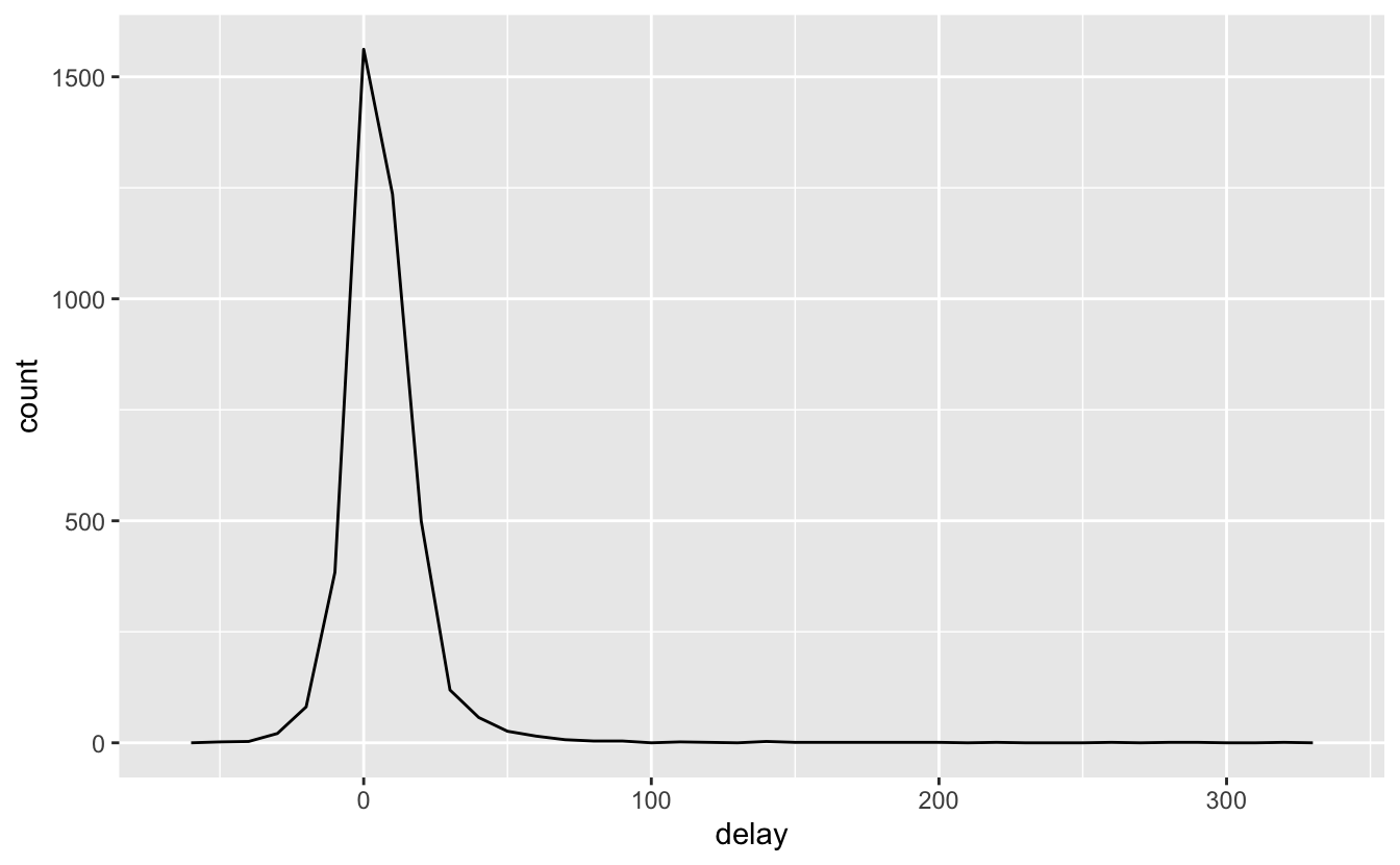

우와, 어떤 항공기들은 평균 5시간 (300분) 지연되었다! 이 이야기는 사실 좀 더 복잡한 문제이다. 비행 횟수 대 평균 지연시간의 산점도를 그리면 더 많은 통찰력을 얻을 수 있다:

ggplot(data = delays, mapping = aes(x = n, y = delay)) +
  geom_point(alpha = 1/10)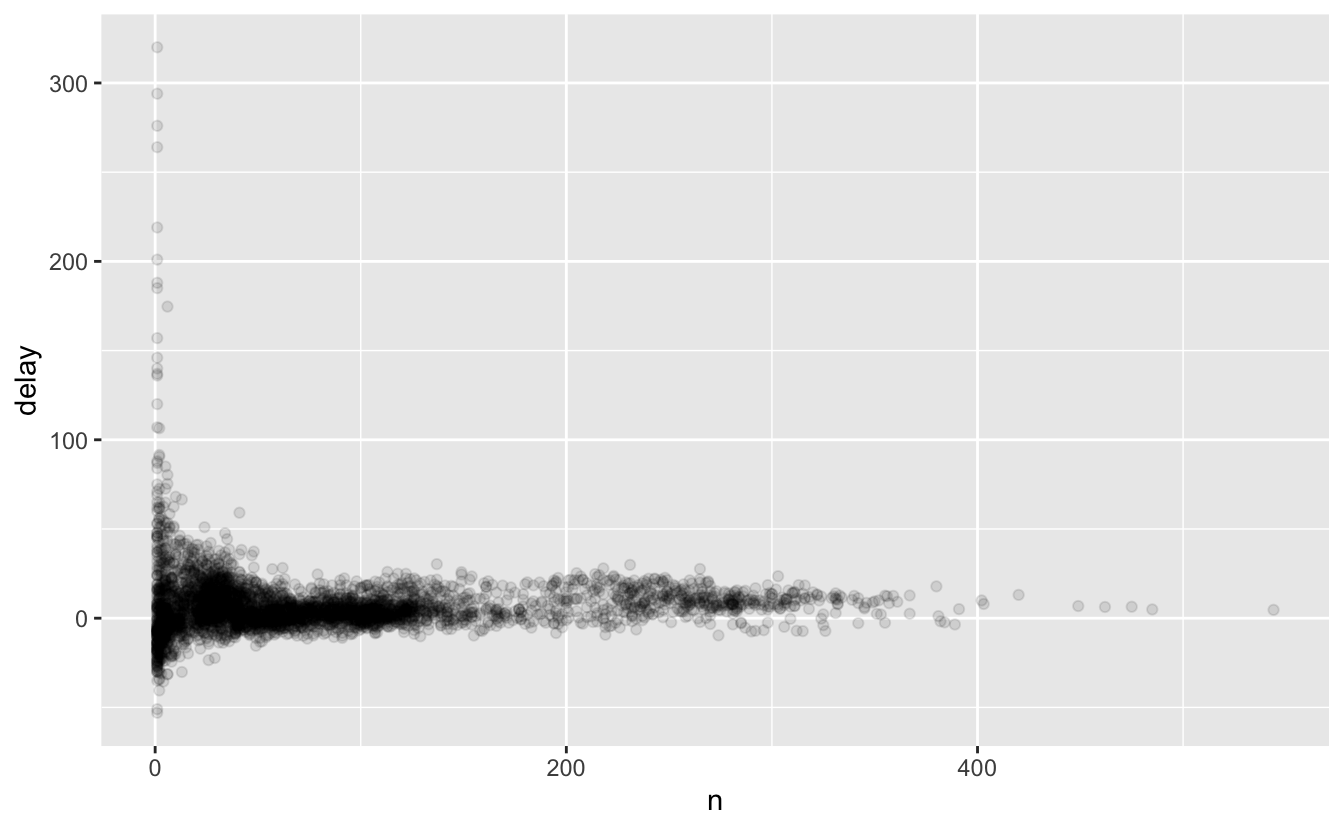

당연히 비행이 적을 때 평균 지연시간에 변동이 훨씬 더 크다. 이 플롯의 모양은 매우 특징적이다. 평균(혹은 다른 요약값) 대 그룹 크기의 플롯을 그리면 표본 크기가 커짐에 따라 변동이 줄어드는 것을 볼 수 있다.

이런 종류의 플롯을 살펴볼 때는, 관측값 개수가 가장 적은 그룹을 필터링하는 것이 좋은 경우가 많다. 심한 변동이 아닌 패턴이 더 잘 보이기 때문이다. 이를 수행하는 다음 코드는 ggplot2 를 dplyr 플로우에 통합하는 편리한 패턴도 보여준다. %>% 에서 + 로 전환해야 한다는 것은 조금 고통스러운 일이지만, 일단 요령을 터득하면 꽤 편리하다.

delays %>%
  filter(n > 25) %>%
  ggplot(mapping = aes(x = n, y = delay)) +
  geom_point(alpha = 1/10) +
  geom_smooth(se = FALSE)
#> `geom_smooth()` using method = 'gam' and formula 'y ~ s(x, bs = "cs")'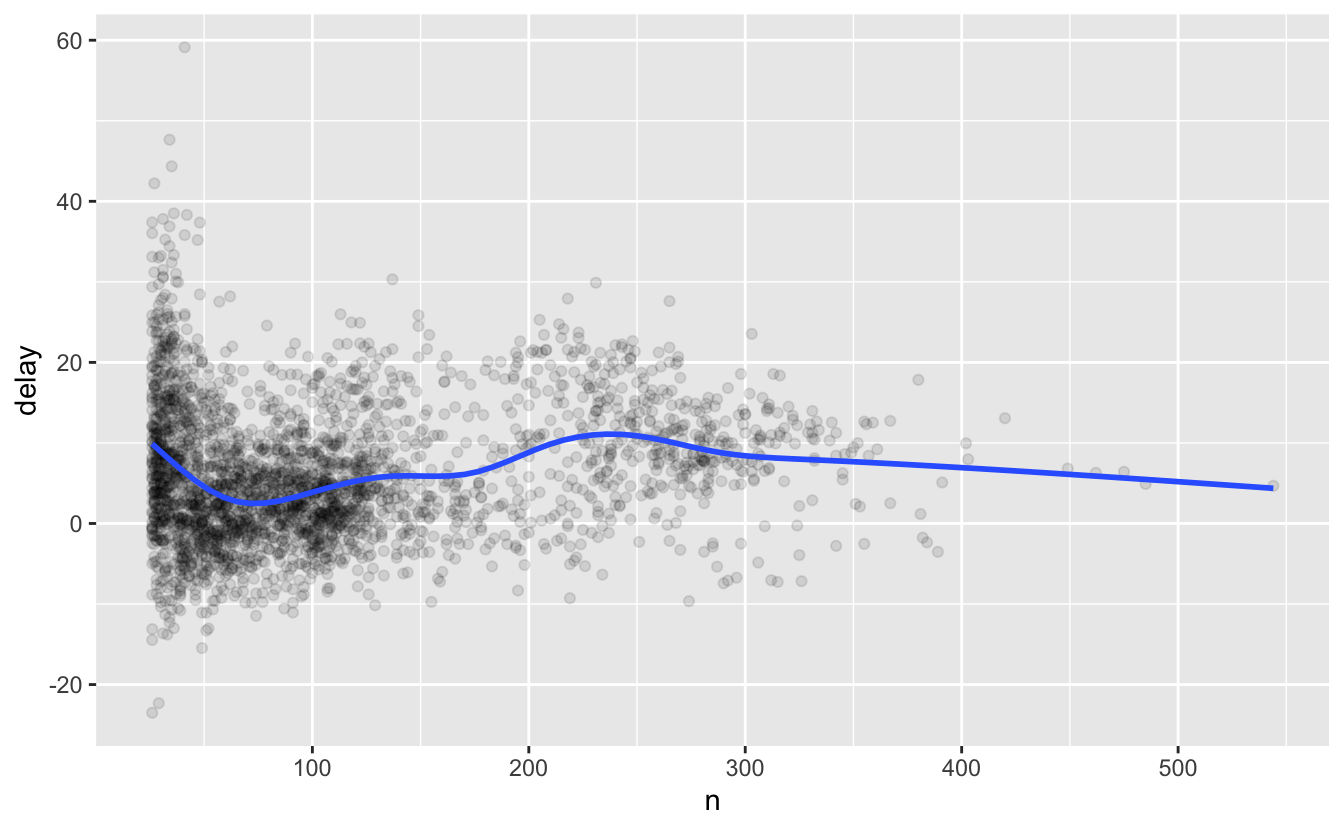

이와 비슷한 유형도 자주 볼 수 있다. 야구에서 타자의 평균 능력치가 타석 수와 어떻게 관련되었는지 살펴보자. 여기에서 Lahman 패키지 데이터를 사용하여 메이저리그의 모든 야구 선수의 타율(안타수/유효타석수)을 계산한다.

batters <- Lahman::Batting %>% 
  group_by(playerID) %>% 
  summarise(
    ba = sum(H, na.rm = TRUE) / sum(AB, na.rm = TRUE),
    ab = sum(AB, na.rm = TRUE)
  )
batters
#> # A tibble: 19,898 × 3
#>   playerID      ba    ab
#>   <chr>      <dbl> <int>
#> 1 aardsda01 0          4
#> 2 aaronha01 0.305  12364
#> 3 aaronto01 0.229    944
#> 4 aasedo01  0          5
#> 5 abadan01  0.0952    21
#> 6 abadfe01  0.111      9
#> # … with 19,892 more rows

타자의 기술(타율, ba 로 측정)을 안타 기회 횟수(타석수, ab 로 측정) 에 대해 플롯을 그리면 두 가지 패턴이 보인다.

1. 앞에서와 같이 집계값의 변동량은 데이터 포인트가 많아짐에 따라 감소한다.

2. 기술 수준(ba)과 볼을 칠 기회(ab) 사이에 양의 상관관계가 있다. 팀이 누구를 타석에 내보낼지 선택할 때 당연히 최고의 선수를 선택할 것이기 때문이다.

batters %>%
  filter(ab > 100) %>%
  ggplot(mapping = aes(x = ab, y = ba)) +
  geom_point(alpha = 1 / 10) +
  geom_smooth(se = FALSE)
#> `geom_smooth()` using method = 'gam' and formula 'y ~ s(x, bs = "cs")'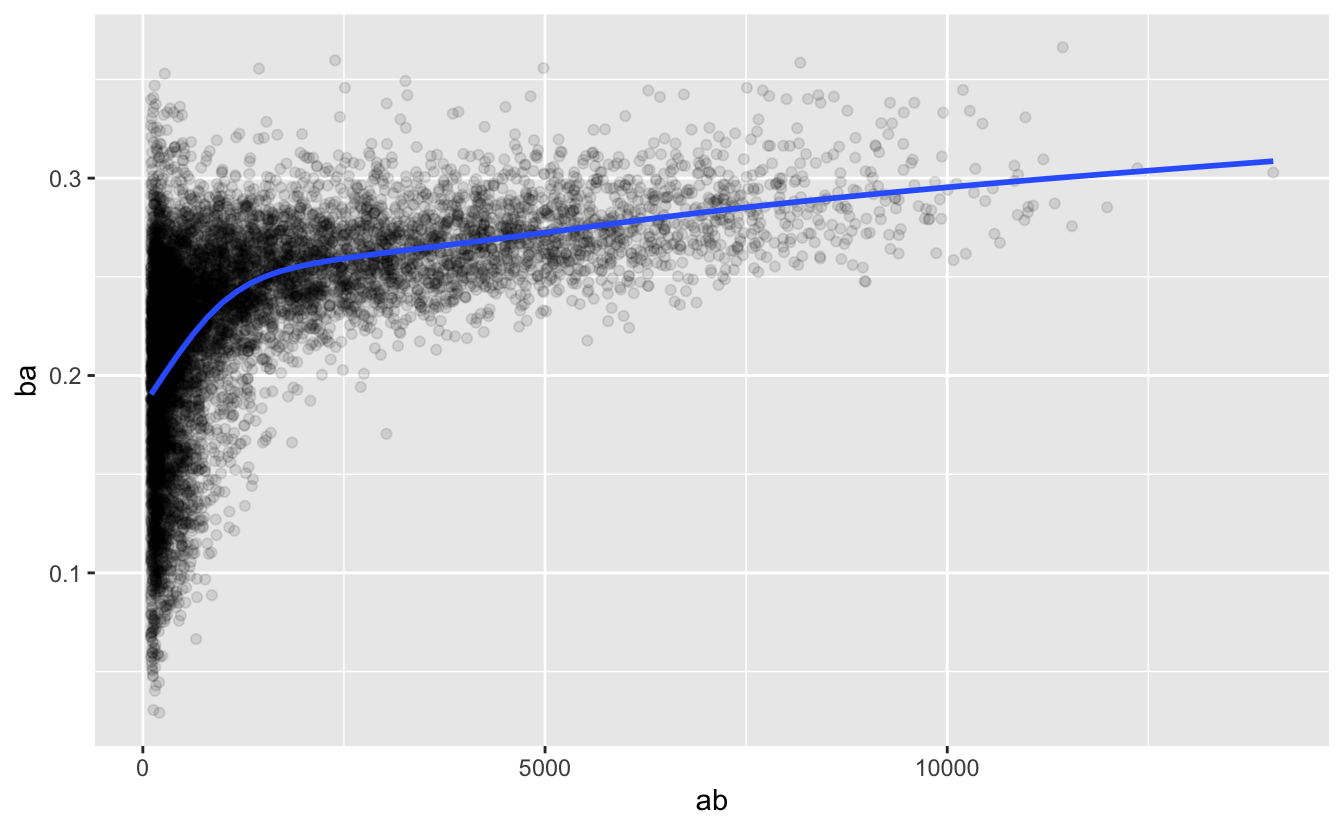

이 사실은 랭킹에 관해 중요한 시사점을 제공한다. 단순히 desc(ba) 로 정렬하면 평균 타율이 가장 높은 선수는 능력치가 좋은 것이 아니라 단순히 운이 좋은 선수들이다.

batters %>%
  arrange(desc(ba))
#> # A tibble: 19,898 × 3
#>   playerID     ba    ab
#>   <chr>     <dbl> <int>
#> 1 abramge01     1     1
#> 2 alanirj01     1     1
#> 3 alberan01     1     1
#> 4 banisje01     1     1
#> 5 bartocl01     1     1
#> 6 bassdo01      1     1
#> # … with 19,892 more rows

다음 사이트에 이 문제에 관해 설명이 잘 되어 있다: http://varianceexplained.org/r/empirical_bayes_baseball/, http://www.evanmiller.org/how-not-to-sort-by-average-rating.html.