Part 11 R Bootcamp
Author: Scott Rodilitz
This document will help you become familiar with (a) how to load data, (b) how to summarize data, and (c) how to visualize data. You are encouraged to use this document as a reference throughout the quarter.
To highlight the power of R, we will examine the association between movie genre and profitability. We will use data on movies from The Numbers and OpusData. The movies included in our dataset were produced between 2006 and 2018 with a production budget greater or equal to $10 million. We will consider movies from six different genres: Action/Adventure, Comedy, Horror, Drama, Thriller, RomCom.
11.1 R Basics
11.1.1 R, RStudio, and R Markdown
We will be using RStudio for this course, which is an interface that helps run R code. If you have this file open in RStudio, you should see four panels.
- In the top left panel, you should see the open files.
- In the bottom left panel, you should see the console, where you can directly type code and view output.
- In the top right panel, you should see any datasets or variables that you have saved during this R session.
- In the bottom right panel, you should see a list of files in your directory. You can also display graphs in this panel.
This file is an R Markdown document. Markdown is a simple formatting syntax for combining R code with written explanations. For more details on using R Markdown see http://rmarkdown.rstudio.com. R Markdown allows you to run code line-by-line, as we will do in this walkthrough, but you can also run the code all at once while creating an .html or .pdf file. To do so, click “knit” at the top of this panel.
11.1.2 Coding in R
11.1.2.1 Code Chunks
Any R code in a Markdown file is embedded in a “chunk” like this:
## [1] 4or this:
## [1] 43219.42To run a code chunk, you can click the little green arrow in the top right corner of the chunk. Alternatively, you can put your cursor anywhere in the chunk and hit ctrl + shift + enter (on Windows) or command + shift + return (on Mac).
You can also run the code line by line. Click into the dropdown menu after “Run” at the top of this panel to see the available options.
An important part of any coding language is commenting. Commenting serves two purposes: (1) To give us little reminders or descriptions about the code, and (2) temporarily ignoring code when we don’t want to run it. For example:
11.1.2.2 Variables and Functions
R allows us to define variables using either <- or =. A variable in R is an extremely flexible “container” that can store the results of calculations, data, plots, and so on.
In the line above, we have defined the variable x to store the result of 2 + 2. Let’s now run a function, also known as a command:
## [1] 4As you would expect, the print() function tells the computer to print anything inside the parentheses. Variables and commands are the pillars of coding in R – we will see many different examples throughout the course.
R can also handle sentences:
## [1] "Welcome to Anderson"As before, we can create a variable to store a sentence:
## [1] "Welcome to Anderson!"After running the code to this point, you should see phrase and x listed in the top right panel of RStudio. This means that those variables are saved for future use. For example, because x is saved in R, we can use it throughout the session:
## [1] 9Be careful about over-writing variables, though. The following code stores a new phrase as phrase and removes its previous definition. Note that we use <- instead of = when defining phrase. The two are equivalent in R, so you may see both from time to time.
## [1] "This is a new phrase."Note that R is case sensitive:
## [1] 4## Error in h(simpleError(msg, call)): error in evaluating the argument 'x' in selecting a method for function 'print': object 'X' not foundYou can clear all variables from the R session by running the “remove” command rm():
11.1.2.3 Vectors
In addition to defining individual variables, we can define a list of variables called a vector. To do so, we need to combine individual variables using the command c. See the examples below:
# Creating a vector of words
word_vector = c("This", "is", "a", "vector", "of", "words")
# Creating a vector of numbers
number_vector = c(9, 16, 2022)
# Printing a vector
print(word_vector)
## [1] "This" "is" "a" "vector" "of" "words"## [1] 9 16 2022If you are ever confused about a specific command, feel free to ask R for help using the help command:
11.1.2.4 Data Frames
Single-dimensional data can be stored as a vector, but more complex data is stored as a Data Frame. A data frame is comparable to an Excel spreadsheet. Most of the time, we will create data frames in R by importing large amounts of data. (More on this later.) However, you can also create a date frame manually using the command data.frame:
# Creating a data frame
PROFESSORS = data.frame(FirstName = c("Auyon", "Scott"), LastName = c("Siddiq", "Rodilitz"), NumSections = c(3,2))

# Printing the data frame
print(PROFESSORS)
## FirstName LastName NumSections
## 1 Auyon Siddiq 3
## 2 Scott Rodilitz 2The code above manually creates the data frame **PROFESSORS*. In general, we will be reading in datasets to create data frames.
11.1.2.5 Installing and Loading Packages
R is open source, which means that are many add-on packages that have been built by members of the R community to make life easier. We are going to start with one package, tidyverse, which is a collection of smaller packages for working with data.
Before using a package, we first need to install it. Installing a package can take a few minutes. Luckily, because we are using RStudio in the cloud, we pre-installed the requisite packages for this course for you.
Since we do not need to install the package, we have used the # symbol to turn the command into a comment. If you did need to install the package, you could delete the # symbol and run the code.
Any time you want to use a package, you will need to load it. This is much faster than installing.
11.2 Working with Data
11.2.1 Importing Data
Before analyzing any data in R, we need to import it. Note that you may need to change the file path to successfully import the file. We will name the dataset MOVIES.
Here we have saved the dataset under the name MOVIES. By default, the read.csv() function saves the dataset as a dataframe in R. Whenever we want to do something with the dataset, we will use the name that we gave it. Note .csv refers to “comma separated values”, which is the standard format for data organized into a table.
If you attempt to load a file using the wrong file path, you will get an error:
## Warning in file(file, "rt"): cannot open file '402/MovieData.csv': No such file
## or directory
## Error in file(file, "rt"): cannot open the connectionWe can also import data directly from a .csv file hosted online. In this course, we will often provide you with the URLs that you can fetch the data from for simplicity:
## Warning in file(file, "rt"): cannot open file 'URL': No such file or directory## Error in file(file, "rt"): cannot open the connection11.2.2 Inspecting Data
You should always inspect a dataset after importing it, to see all of the variables it contains (also known as the features). This also ensures that the data is what you expect. Here are some ways to do this.
11.2.2.1 Viewing data
Open a window to view the data (akin to opening the file in Excel). Currently, the command below is commented out using the # symbol. In other words, the computer will ignore the command. If you remove the # symbol and run the code, it will open a new tab in this panel of RStudio, which you will need to close.
To print the first few rows of data, also known as the head of the dataset, we can run the following command:
##            Title Year   Budget DomesticBoxOffice TotalBoxOffice    Rating
## 1         Krrish 2006 10000000           1430721       32430721 Not Rated
## 2          Crank 2006 12000000          27838408       43924923         R
## 3     The Marine 2006 15000000          18844784       22165608     PG-13
## 4 Running Scared 2006 17000000           6855137        9729088         R
## 5    Renaissance 2006 18000000             70644        2401413         R
## 6     BloodRayne 2006 25000000           2405420        3711633         R
##                Source            Method            Genre Sequel Runtime
## 1 Original Screenplay       Live Action Action/Adventure      1      NA
## 2 Original Screenplay       Live Action Action/Adventure      0      88
## 3 Original Screenplay       Live Action Action/Adventure      0      NA
## 4 Original Screenplay       Live Action Action/Adventure      0      NA
## 5 Original Screenplay Digital Animation Action/Adventure      0     105
## 6       Based on Game       Live Action Action/Adventure      0      92
11.2.2.2 Counting rows
To count the number of rows (also known as observations, or movies in this example), you can use the following command, or simply look at the list of datasets in the top right panel.
## [1] 187511.2.2.3 Listing variables/columns
List the columns (also known as the variables or the features) included in the dataset:
##  [1] "Title"             "Year"              "Budget"
##  [4] "DomesticBoxOffice" "TotalBoxOffice"    "Rating"
##  [7] "Source"            "Method"            "Genre"
## [10] "Sequel"            "Runtime"
You can also print the structure (i.e., variable type) of each column along with the first few entries.
## 'data.frame':    1875 obs. of  11 variables:
##  $ Title            : chr  "Krrish" "Crank" "The Marine" "Running Scared" ...
##  $ Year             : int  2006 2006 2006 2006 2006 2006 2006 2006 2006 2006 ...
##  $ Budget           : int  10000000 12000000 15000000 17000000 18000000 25000000 30000000 30000000 40000000 40000000 ...
##  $ DomesticBoxOffice: int  1430721 27838408 18844784 6855137 70644 2405420 18522064 669625 659210 50866635 ...
##  $ TotalBoxOffice   : num  32430721 43924923 22165608 9729088 2401413 ...
##  $ Rating           : chr  "Not Rated" "R" "PG-13" "R" ...
##  $ Source           : chr  "Original Screenplay" "Original Screenplay" "Original Screenplay" "Original Screenplay" ...
##  $ Method           : chr  "Live Action" "Live Action" "Live Action" "Live Action" ...
##  $ Genre            : chr  "Action/Adventure" "Action/Adventure" "Action/Adventure" "Action/Adventure" ...
##  $ Sequel           : int  1 0 0 0 0 0 0 0 0 0 ...
##  $ Runtime          : int  NA 88 NA NA 105 92 NA NA NA 138 ...
The basic data types you will usually encounter are chr (character, i.e., text) for categorical variables, and int (integer) or num (number, which may include decimals) for numerical variables.
11.2.2.4 Summarizing a variable
To investigate a particular variable, you first list the dataset, then the $ symbol, then the variable name. For quantitative variables, you may want to calculate the mean or the standard deviation. The command “summary” also gives some good information:
## [1] 53425611## [1] 53586268## Min. 1st Qu. Median Mean 3rd Qu. Max.
## 10000000 19450000 33000000 53425611 65000000 425000000Note that the standard deviation and the mean are quite close to each other. This suggests that there is a lot of variability in movie budgets, even among these movies which all have budgets over $10 million.
For categorical variables, “summary” is pretty useless:
##    Length     Class      Mode
##      1875 character character
Instead, the command “table” provides the information we would want.
##
##                   G     NC-17 Not Rated        PG     PG-13         R
##        19        30         1        38       295       762       730
The most common rating in the database Note that there are 38 movies which are listed as “Not Rated” and an additional 19 movies for which no information is provided.
11.2.2.5 Summarizing the dataset
We can also generate a summary of the entire data frame, including the data type and a numerical summary.
##     Title                Year          Budget          DomesticBoxOffice
##  Length:1875        Min.   :2006   Min.   : 10000000   Min.   :        0
##  Class :character   1st Qu.:2008   1st Qu.: 19450000   1st Qu.: 11349430
##  Mode  :character   Median :2011   Median : 33000000   Median : 36661504
##                     Mean   :2011   Mean   : 53425611   Mean   : 64217975
##                     3rd Qu.:2014   3rd Qu.: 65000000   3rd Qu.: 79920496
##                     Max.   :2018   Max.   :425000000   Max.   :936662225
##
##  TotalBoxOffice         Rating             Source             Method
##  Min.   :3.471e+03   Length:1875        Length:1875        Length:1875
##  1st Qu.:2.687e+07   Class :character   Class :character   Class :character
##  Median :7.380e+07   Mode  :character   Mode  :character   Mode  :character
##  Mean   :1.592e+08
##  3rd Qu.:1.801e+08
##  Max.   :2.776e+09
##
##     Genre               Sequel          Runtime
##  Length:1875        Min.   :0.0000   Min.   :  0.0
##  Class :character   1st Qu.:0.0000   1st Qu.: 97.0
##  Mode  :character   Median :0.0000   Median :108.0
##                     Mean   :0.1559   Mean   :109.4
##                     3rd Qu.:0.0000   3rd Qu.:120.0
##                     Max.   :1.0000   Max.   :201.0
##                     NA's   :2        NA's   :105
11.2.3 Cleaning and Managing Data
You may have noticed that some data appear to be missing. Using the code below, we can remove all movies with any missing numerical entries, shown as NA in the summary above. This avoids errors later on (e.g., when calculating averages). Before doing so, it’s always good to think about WHY the entries are missing.
11.2.3.2 Selecting rows
Sometimes, you may only want a portion of your data. If you only want some of the rows, you can use the subset function. Here, we are selecting only the films where the genre is listed as “Horror”. Note that we use two equal signs when we are asking the computer to check for equality.
HORROR = subset(MOVIES, Genre == "Horror")

# How many are there?
# If we had a typo, there would be 0.
# If we used a single equal sign, it would include ALL movies
nrow(HORROR)
## [1] 9211.2.3.3 Selecting columns
If you only want some of the columns, you can use the select function:
##           Title Year            Genre
## 2         Crank 2006 Action/Adventure
## 5   Renaissance 2006 Action/Adventure
## 6    BloodRayne 2006 Action/Adventure
## 10   Apocalypto 2006 Action/Adventure
## 13    16 Blocks 2006 Action/Adventure
## 15 The Guardian 2006 Action/Adventure
11.2.4 Creating New Variables
Before we investigate which genre of movie provides the best return on investment (ROI), we need to compute those values for each movie! Luckily, this is easy to do with a single line of code:
Note that if you fund a movie with an ROI of 1, you have doubled your money.
11.2.5 Common Errors
Using R can be tricky! Computers need precise instructions. Small typos can lead to errors. Often, the error message can give some clue as to what went wrong, as shown by these examples.
If you attempt to load a file using the wrong file path, you will get an error:
## Warning in file(file, "rt"): cannot open file '402/MovieData.csv': No such file
## or directory
## Error in file(file, "rt"): cannot open the connectionAnother reminder: R is case sensitive! Using Movies instead of the correct form MOVIES will return an error:
## Error in h(simpleError(msg, call)): error in evaluating the argument 'object' in selecting a method for function 'summary': object 'Movies' not foundIf you want to access a variable without referencing its dataset, you will get an error.
## Error in h(simpleError(msg, call)): error in evaluating the argument 'object' in selecting a method for function 'summary': object 'Year' not foundIf you get stuck on an error, try asking an AI model like ChatGPT or Microsoft CoPilot. Check the “CODE” tutorial on BruinLearn for more about troubleshooting coding errors with AI.
11.3 Analyzing Data
11.3.1 Including Plots
Visualizing data is one of the best ways to understand patterns and generate insights. In an R Markdown document, you can create and embed plots, for example:
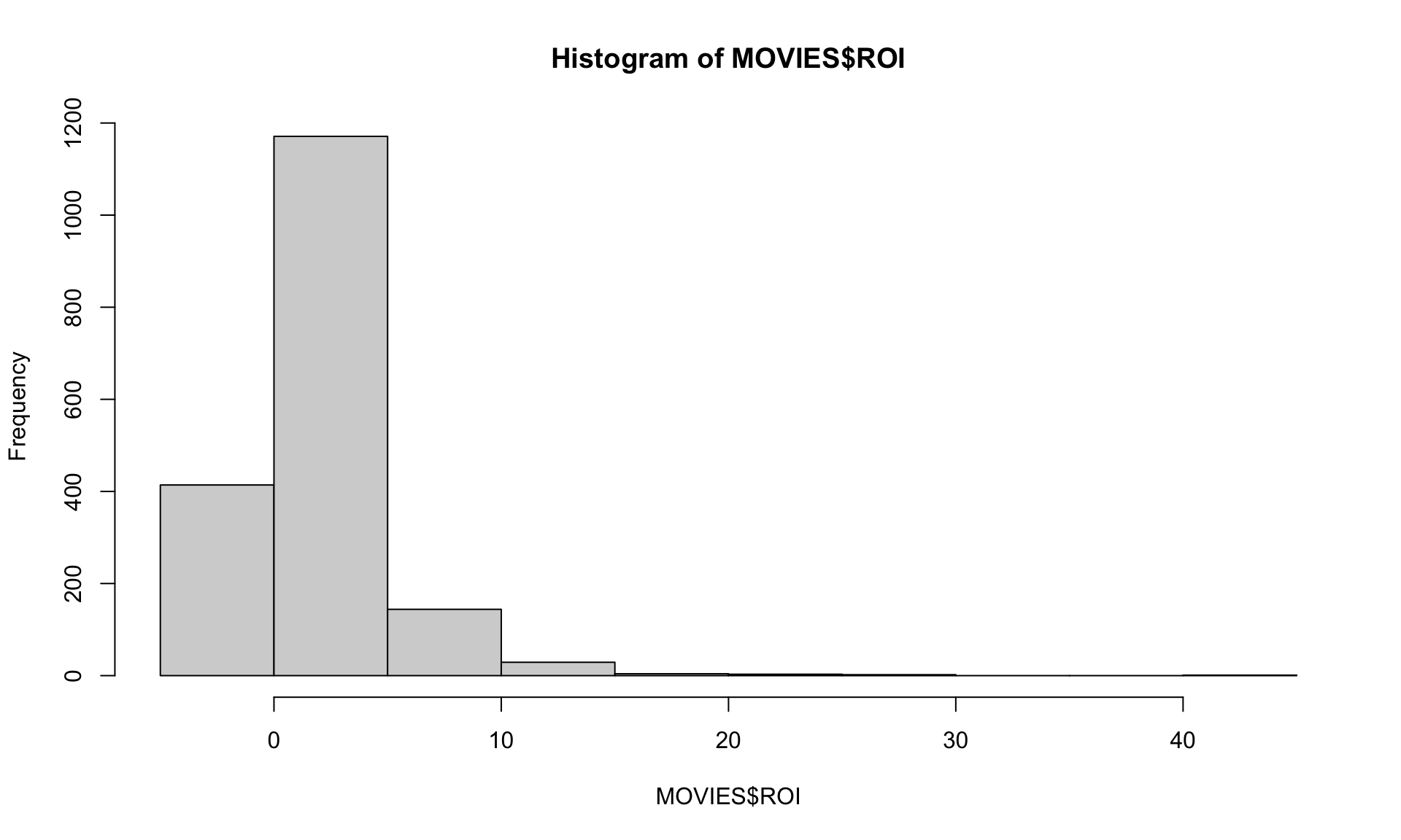
You can also view plots in the bottom right panel of RStudio. To make this the default behavior, click the “settings wheel” icon to the right of Knit (above). Select “Chunk Output in Console”.
This is a histogram. Each bar (usually referred to as a “bin”) displays the total count of movies with an ROI between the left and right end points of the bar. For example, about 400 movies had a negative ROI. Unfortunately, the bins are a bit too wide to tell a clear story. (What is the lowest possible ROI?)
To improve the histogram, we can add some optional arguments to the command hist. Let’s manually create narrower bins, using the argument “breaks”. We can also narrow the range of values that we see in the plot using the argument “xlim”, and we can make the plot a bit prettier by adding color with the argument “col”.
options(warn=-1)
hist(MOVIES$ROI, breaks = c(-1,0, 1, 2, 3, 4, 5, 6, 7, 8, 50),
     xlim = c(-1,8), col = 'red')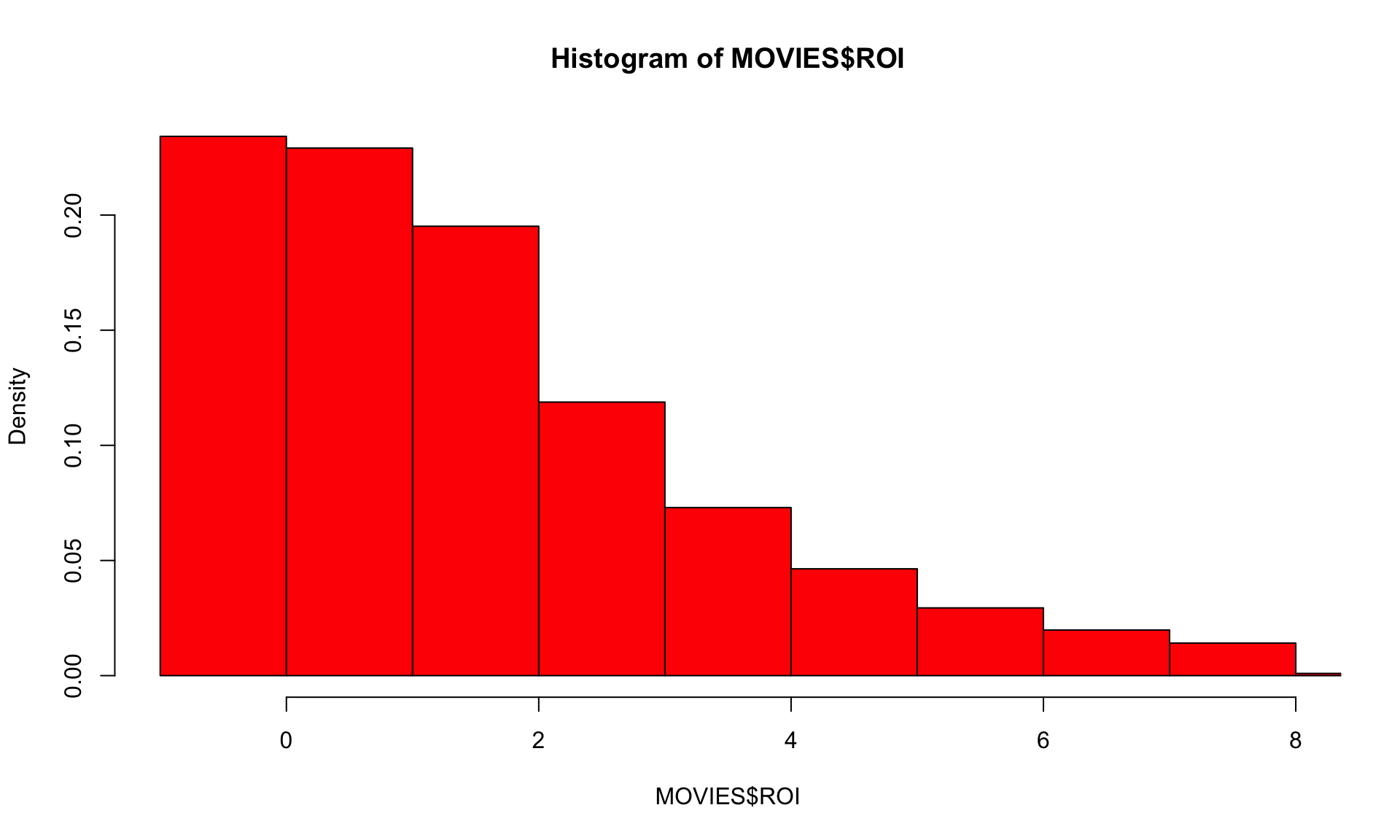
This plot lumps together anything with an ROI over 8, and mostly hides that bin in the plot using the “xlim” command. To answer questions like “what percent of movies lose money?” we can look at the same plot, but with proportions instead of frequency counts, using the “freq” argument. By default, freq = TRUE, but we can change that:
options(warn=-1)
hist(MOVIES$ROI, breaks = c(-1,0, 1, 2, 3, 4, 5, 6, 7, 8, 50),
     xlim = c(-1,8), col = 'green', freq = FALSE)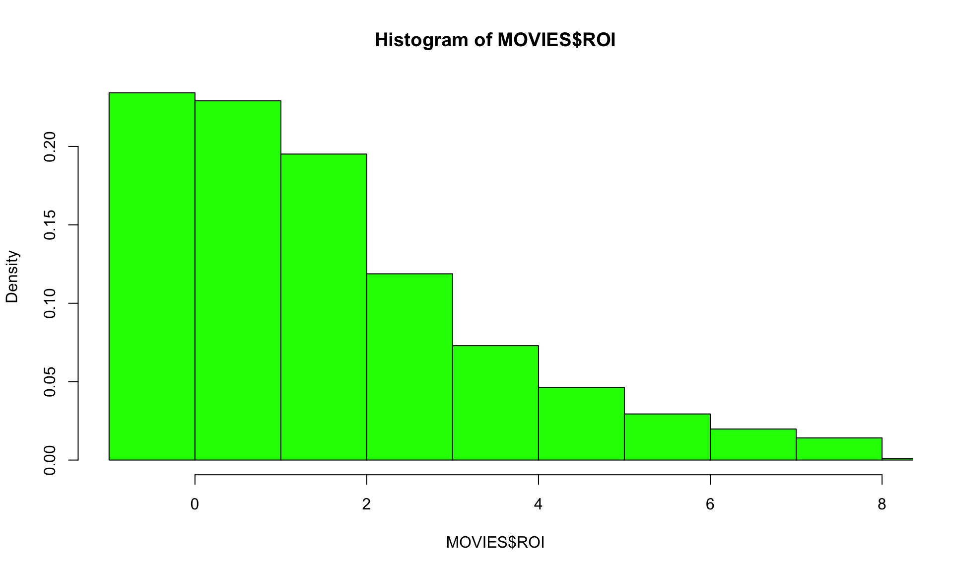
We can also look at a boxplot, which gives information about the distribution of ROI:
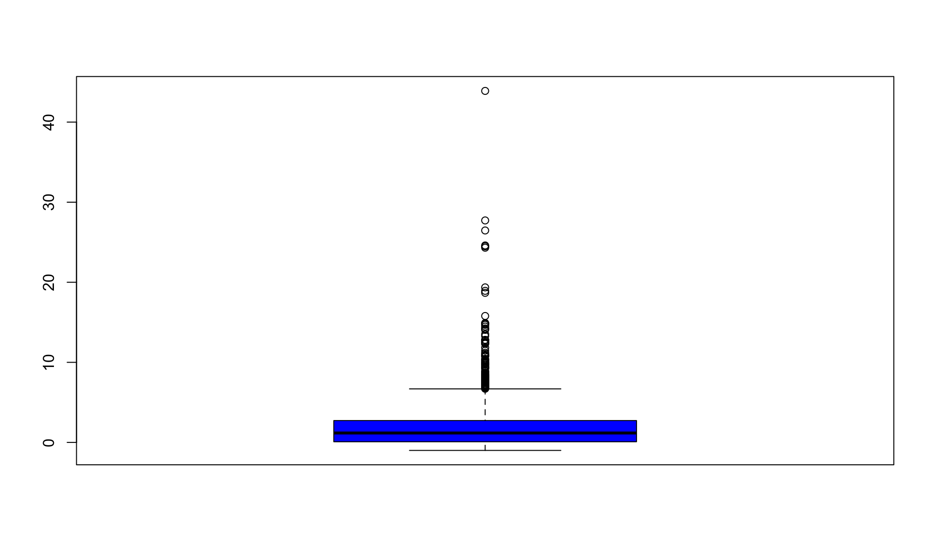
The solid black line is the median. Half of the movies have an ROI between the top and bottom of the box (the 75th and 25th percentiles).
11.3.2 Identifying Outliers
Anything above (or below) the “whiskers” of the box are considered outliers, at least by some definitions. Sometimes, it can make sense to remove outliers before analyzing the data. At the very least, it is good to investigate them to make sure there aren’t any data errors. We can look at the movies with the highest ROI using the following command:
##                    Title Year   Budget DomesticBoxOffice TotalBoxOffice Rating
## 1       Les Intouchables 2011 10800000          13182281      484873045      R
## 2    The King’s Speech 2010 15000000         138797449      430821168      R
## 3    Slumdog Millionaire 2008 14000000         141330703      384530440      R
## 4 The Fault in Our Stars 2014 12000000         124872350      307166834  PG-13
## 5             Black Swan 2010 13000000         106954678      331266710      R
## 6              Halloween 2018 10000000         159342015      253139306      R
##                              Source      Method    Genre Sequel Runtime
## 1               Original Screenplay Live Action   Comedy      0     110
## 2               Original Screenplay Live Action    Drama      0     118
## 3               Original Screenplay Live Action    Drama      0     116
## 4 Based on Fiction Book/Short Story Live Action    Drama      0     125
## 5               Original Screenplay Live Action Thriller      0     108
## 6               Original Screenplay Live Action   Horror      1     105
##        ROI
## 1 43.89565
## 2 27.72141
## 3 26.46646
## 4 24.59724
## 5 24.48205
## 6 24.31393
We can create a new dataset which removes any movie with an ROI above a threshold:
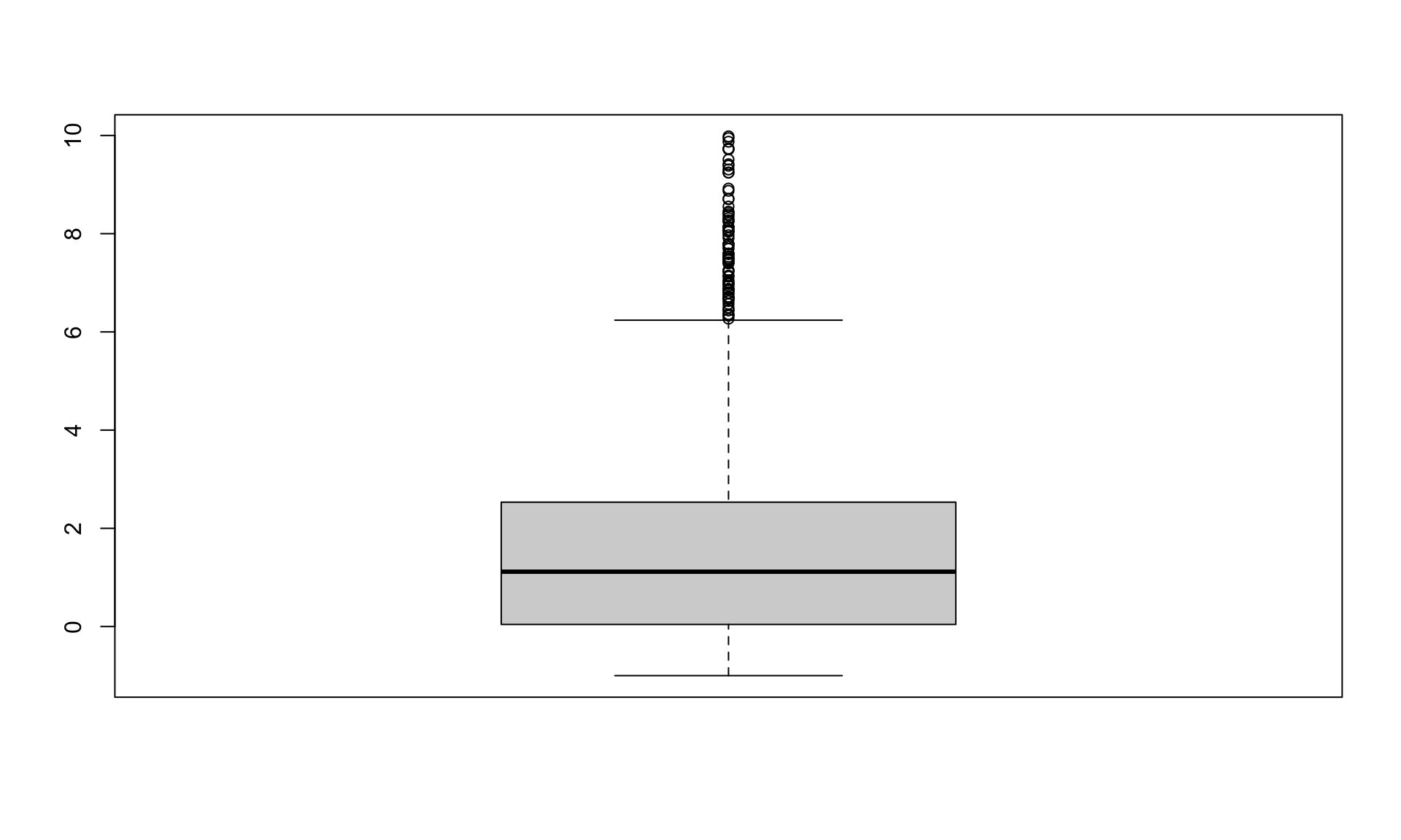
The name of this new dataset, “NO_OUTLIERS” is a bit misleading. There is no universally-accepted rule for what constitutes an outlier. (See https://en.wikipedia.org/wiki/Outlier#Definitions_and_detection for more info.) How to define and handle outliers depends on the context. For today’s exercise, we will use the full dataset.
11.3.3 Grouping by a Variable
We want to figure out which type of movie is likely to generate the most ROI. To investigate, let’s separate our data based on genre, and then generate some summary statistics:
#This creates a new dataset that groups movies based on their genre
MOVIES_BY_GENRE = group_by(MOVIES, Genre)

#This creates a new dataset that has summary statistics for ROI about each genre
ROI_SUMMARY = summarize(MOVIES_BY_GENRE,
                        Mean = mean(ROI), Median = median(ROI), SD = sd(ROI), count = n())

#This displays those summary statistics for the first six genres
#Since our data only includes six genres, this is a complete summary
head(ROI_SUMMARY, 6)
## # A tibble: 6 × 5
## Genre Mean Median SD count
## <chr> <dbl> <dbl> <dbl> <int>
## 1 Action/Adventure 1.91 1.43 2.23 618
## 2 Comedy 2.01 1.18 3.58 318
## 3 Drama 1.63 0.629 3.46 434
## 4 Horror 3.81 1.95 5.15 92
## 5 RomCom 2.08 1.53 2.17 80
## 6 Thriller 1.57 1.01 2.57 226#This plots the means ROI for each genre.
#If you are curious: The argument ylab = "ROI" labels the y-axis.
# The argument las = 2 makes the x-axis labels vertical.
# The argument col = c(1:6) assigns colors to each bar (1 = black, etc.)
# In that argument, "1:6" means "1 through 6"
barplot(height=ROI_SUMMARY$Mean, names=ROI_SUMMARY$Genre, ylab="ROI", las = 2, col = c(1:6))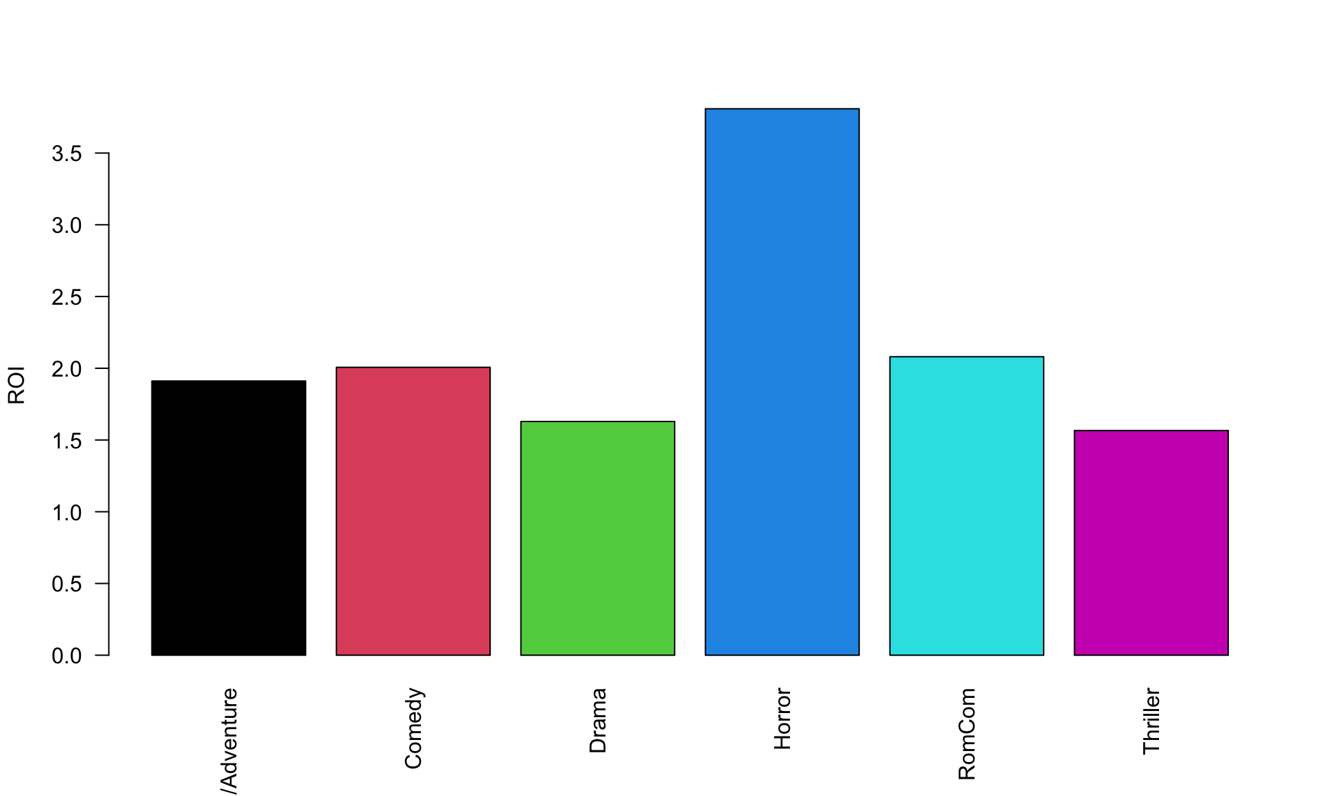
Does this mean horror is the best deal? Well, it depends on your risk tolerance:
#This creates a scatter plot
plot(ROI_SUMMARY$SD, ROI_SUMMARY$Mean, xlim = c(2,6))

#This labels the points. "pos = 4" says to put the labels to the right.
text(ROI_SUMMARY$SD, ROI_SUMMARY$Mean, labels=ROI_SUMMARY$Genre, pos = 4)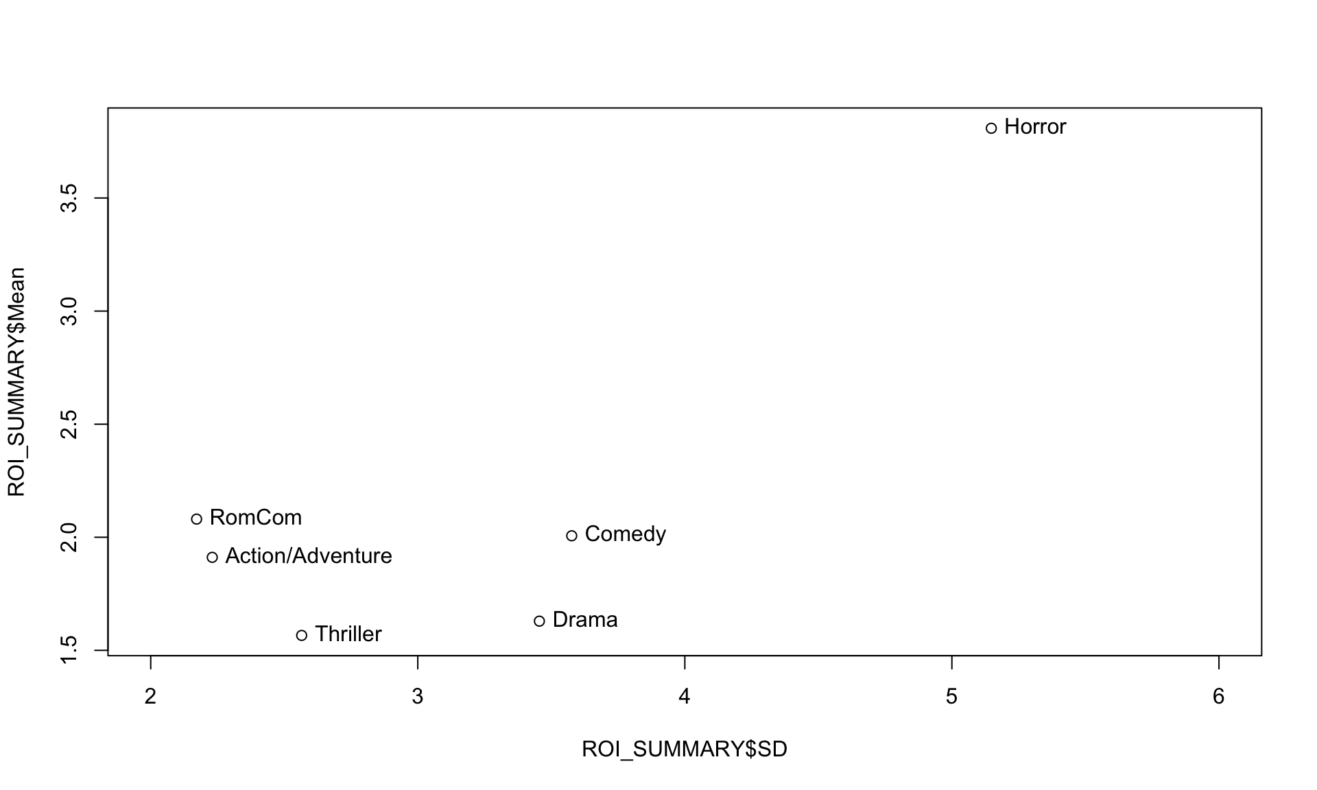
This is a scatter plot which shows one data point for each genre. The standard deviation of ROI for that genre is its position on the x-axis, and the mean ROI for that genre is its height on the y-axis. The second line of code adds labels. Based on this graph, it might make sense to invest in some combination of RomComs and Horror films to maximize ROI but limit risk.
What other differences across genres might we find that could be important parts of the story?
#This creates a new dataset that has summary statistics for Budget about each genre
BUDGET_SUMMARY = summarize(MOVIES_BY_GENRE,
                        Mean = mean(Budget), Median = median(Budget), SD = sd(Budget))

#This displays those summary statistics for all six genres
head(BUDGET_SUMMARY, 6)
## # A tibble: 6 × 4
## Genre Mean Median SD
## <chr> <dbl> <dbl> <dbl>
## 1 Action/Adventure 94514887. 77250000 69092505.
## 2 Comedy 33696541. 27750000 24081599.
## 3 Drama 31717742. 24600000 26198551.
## 4 Horror 27076630. 20000000 24070401.
## 5 RomCom 33369000 30000000 21338177.
## 6 Thriller 41044248. 30000000 32000441.#This plots the means Budget for each genre.
barplot(height=BUDGET_SUMMARY$Mean, names=BUDGET_SUMMARY$Genre,
ylab="Budget", las = 2, col = c(1:6))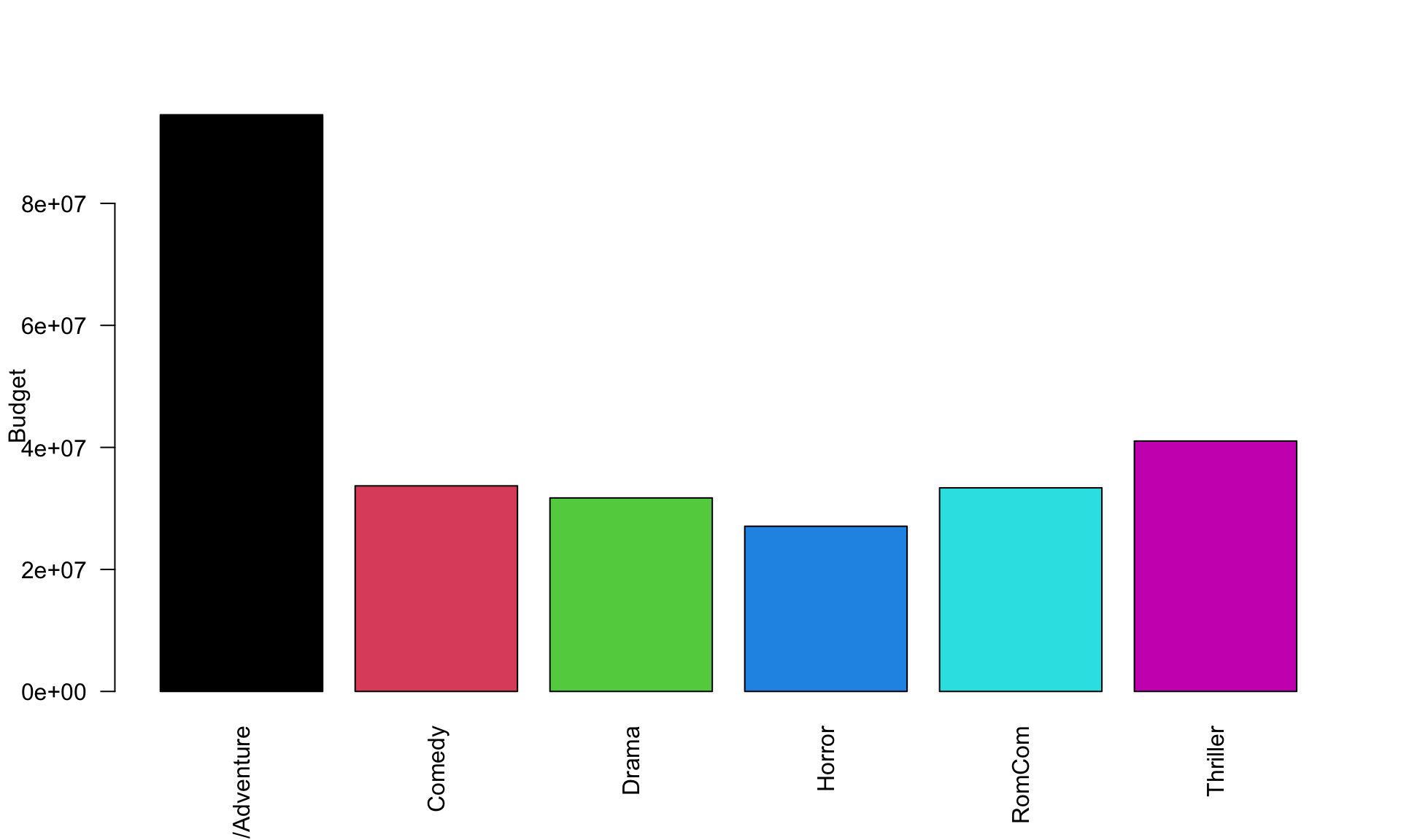
How much does the size of the budget influence ROI? We can investigate this by creating a binary variable. Binary variables are either 0 or 1. Here, we create a variable “LowBudget” which is 1 if a movie has a budget below $20 million, and is 0 otherwise. Then we look for differences in ROI between low-budget and high-budget movies.
#This creates a scatter plot showing the relationship between budget and ROI
plot(MOVIES$Budget, MOVIES$ROI)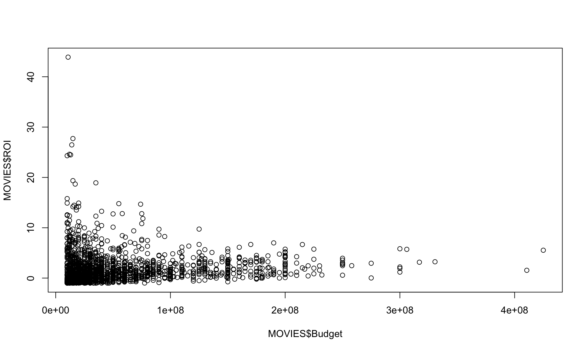
#This creates a new binary variable.
MOVIES$LowBudget = ifelse(MOVIES$Budget<20000000,1,0)

#This separates movies into two groups, based on their budget
MOVIES_BY_BUDGET = group_by(MOVIES, LowBudget)

#This creates a new dataset with summary statistics on ROI separated by budget
ROI_SUMMARY_BY_BUDGET = summarize(MOVIES_BY_BUDGET,
                        Mean = mean(ROI), Median = median(ROI), SD = sd(ROI), count = n())
head(ROI_SUMMARY_BY_BUDGET)
## # A tibble: 2 × 5
## LowBudget Mean Median SD count
## <dbl> <dbl> <dbl> <dbl> <int>
## 1 0 1.76 1.21 2.33 1351
## 2 1 2.43 0.799 4.77 417Why might low-budget movies have a better average ROI? Well, there is some natural limit on how much box office revenue you can generate, even with a huge budget. Hence, you may be more likely to get large ROI on low-budget films. They are also riskier. In fact, the median ROI for a high-budget film is higher than the median ROI for a low-budget film.
11.3.4 Extra Content: Advanced Data Visualization
Usually it is most useful to look at simple charts and figures when investigating data. When attempting to present data in a compelling way, however, it can be useful to create more sophisticated visuals. Creating fancy visuals is not a focus of this course, but it is good to be aware of the possibilities.
There are some packages in R which can help create nice images. We will use one of these packages below called ggplot2. We already loaded this package as part of tidyverse so we do not need to run the command library(ggplot2).
Designing presentation-quality visuals is both an art and a science. It requires much more code than a basic plot. An excellent reference for plotting with pre-written code is available at https://r-graph-gallery.com.
ggplot(data = MOVIES, aes(x = ifelse(ROI>10,10,ROI), fill = Genre)) +
  geom_histogram(color="white", binwidth = 0.5) + facet_wrap(~ Genre) +
  scale_x_continuous("Return on Investment (ROI)", labels = scales::percent)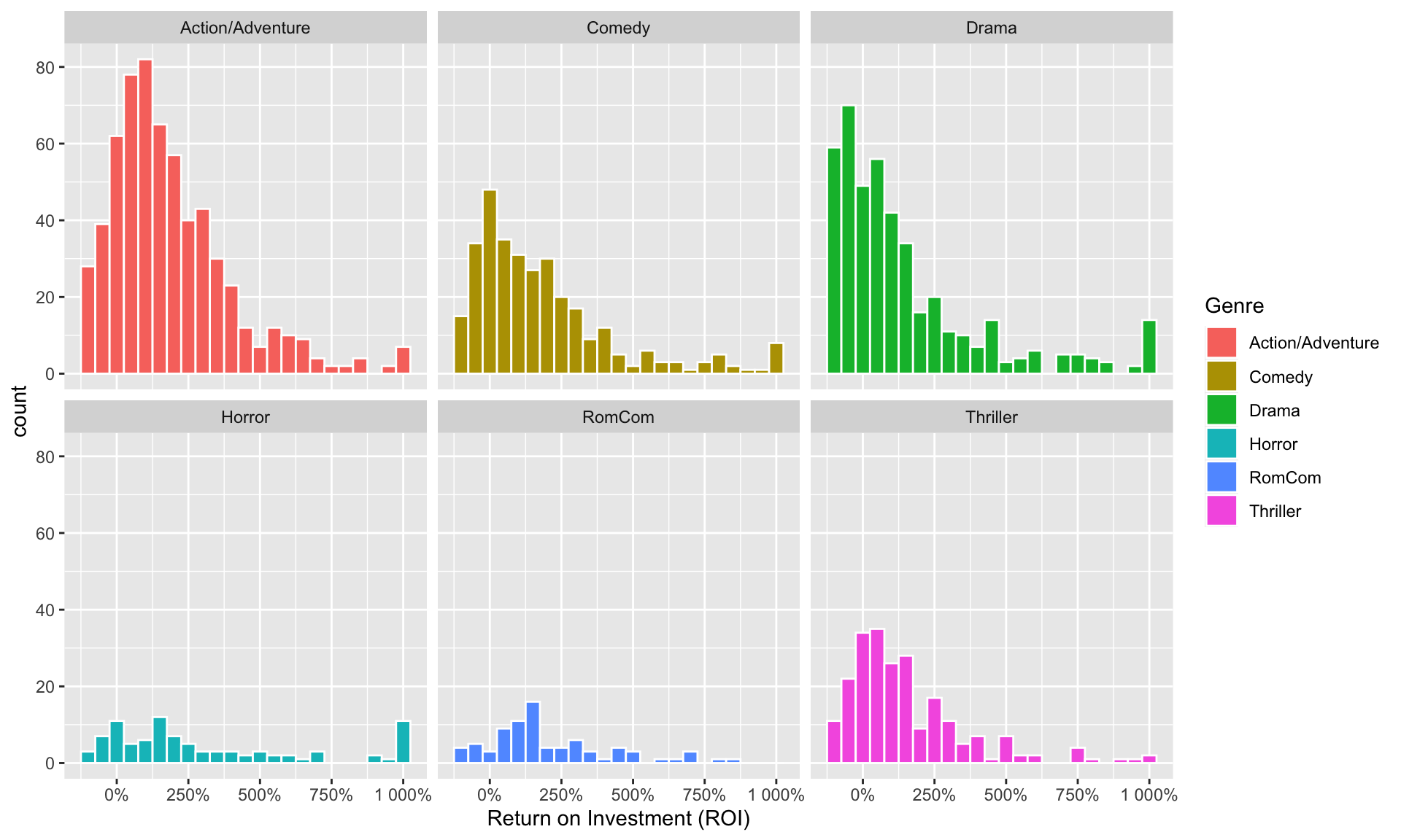
The text in the figure may be a bit large on your computer. To view the figure in a larger window, click “Zoom” in the lower right panel (if your figure shows up there) or click the icon for “Show in New Window” if your figure appears above this text.
The next chunk of code creates a violin plot, which is like a boxplot but it provides a bit more visual information about the distribution.
BUDGET = summarize(group_by(MOVIES, Genre), MeanBudget = mean(Budget))

ggplot(data = MOVIES, aes(x = Genre, y = Budget/1000000, fill = Genre)) +
  geom_violin() +
  stat_summary(fun=mean, geom="crossbar", color="Black") +
  geom_label(data = BUDGET, aes(x = Genre, y = MeanBudget/1000000, label = paste("$", round(MeanBudget/1000000, digits=1))), nudge_y = 10, fill = "White") +
  scale_y_continuous("Budget", labels = scales::dollar_format(prefix="$", suffix = "M"))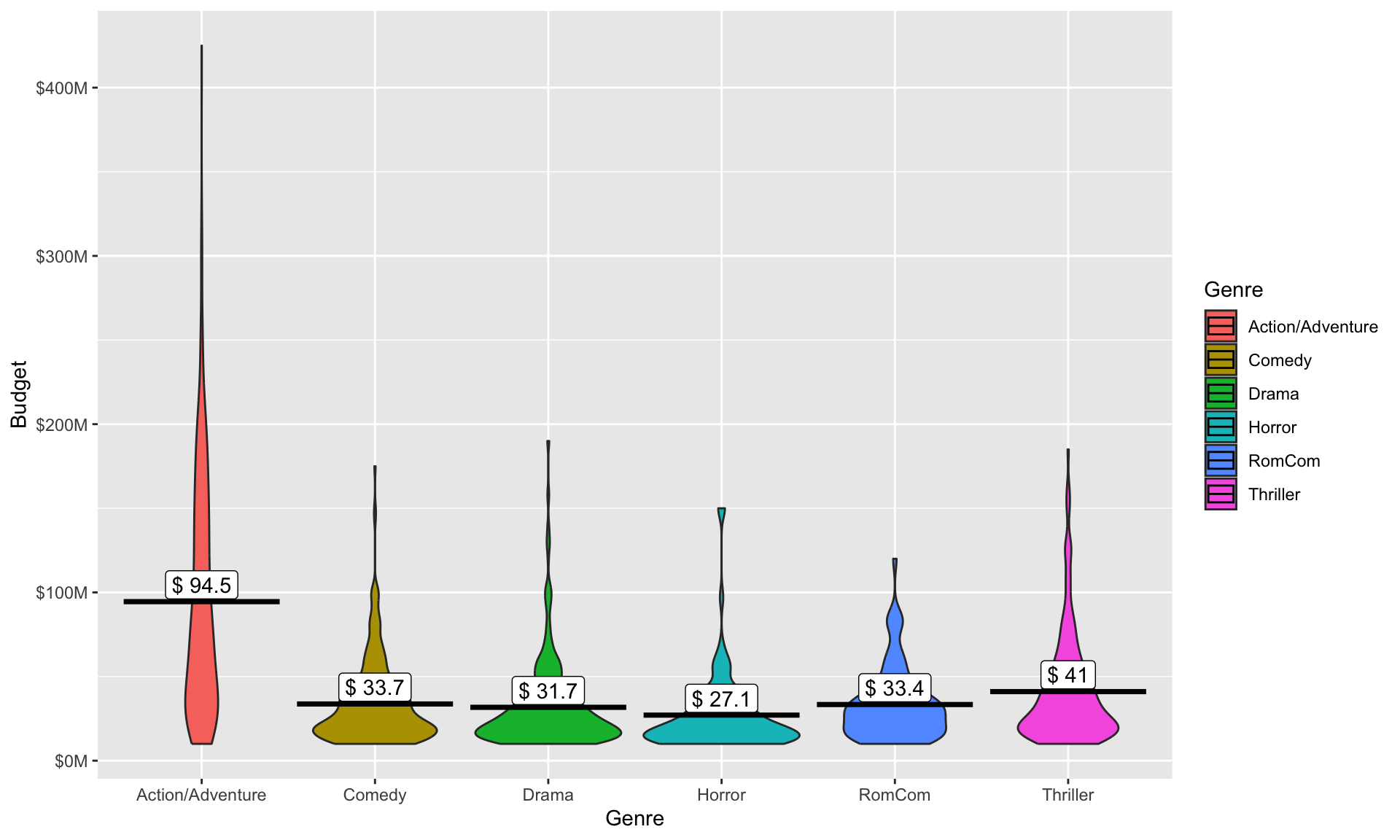
11.4 Course Preview
In the remaining nine weeks, we will build up our data analytics toolkit by asking lots of questions and interacting with many different datasets. However, I hope you remember that the techniques you will learn can also be applied on this original dataset (and many others). See the examples below for a brief preview.
11.4.0.1 Session 2: Probability and Simulation
We can simulate the average ROI from five (equal-budget) horror movies, assuming the ROI for each horror movie is independent and Normally distributed with a mean of 3.81 and a SD of 5.15. (For the record: this is a bad assumption!)
set.seed(1)
ROI_SIM = replicate(n = 1000, rnorm(5, 3.81, 5.15), simplify = TRUE)
summing_ROI = apply(ROI_SIM,2,cumsum)
average_ROI = summing_ROI[5,]/5
hist(average_ROI)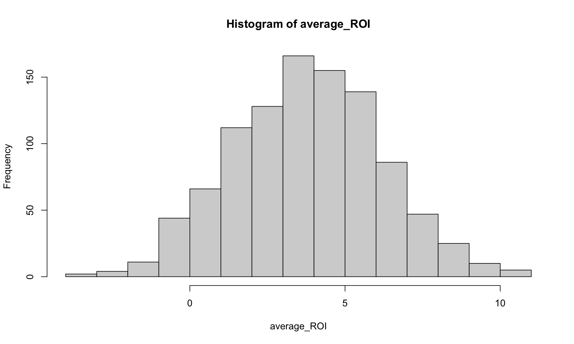
11.4.0.2 Session 3: Sampling and Confidence Intervals
Under the same assumptions as above, we can calculate a 95% right confidence interval for the total ROI:
## [1] 0.0216553411.4.0.3 Session 4: Hypothesis Testing
Is there a significant difference in the mean ROI for horror films and RomComs?
n_1 = 92
mean_1 = 3.81
sd_1 = 5.15
n_2 = 80
mean_2 = 2.08
sd_2 = 2.17
t = (mean_1 - mean_2)/sqrt(sd_1^2/n_1 + sd_2^2/n_2)
2*pnorm(t, lower.tail = FALSE)
## [1] 0.00332243211.4.0.4 Session 5: Linear Regression
Can we predict Box Office revenue from budget?
model = lm(TotalBoxOffice ~ Budget, data = MOVIES)
plot(MOVIES$TotalBoxOffice ~ MOVIES$Budget)
abline(model)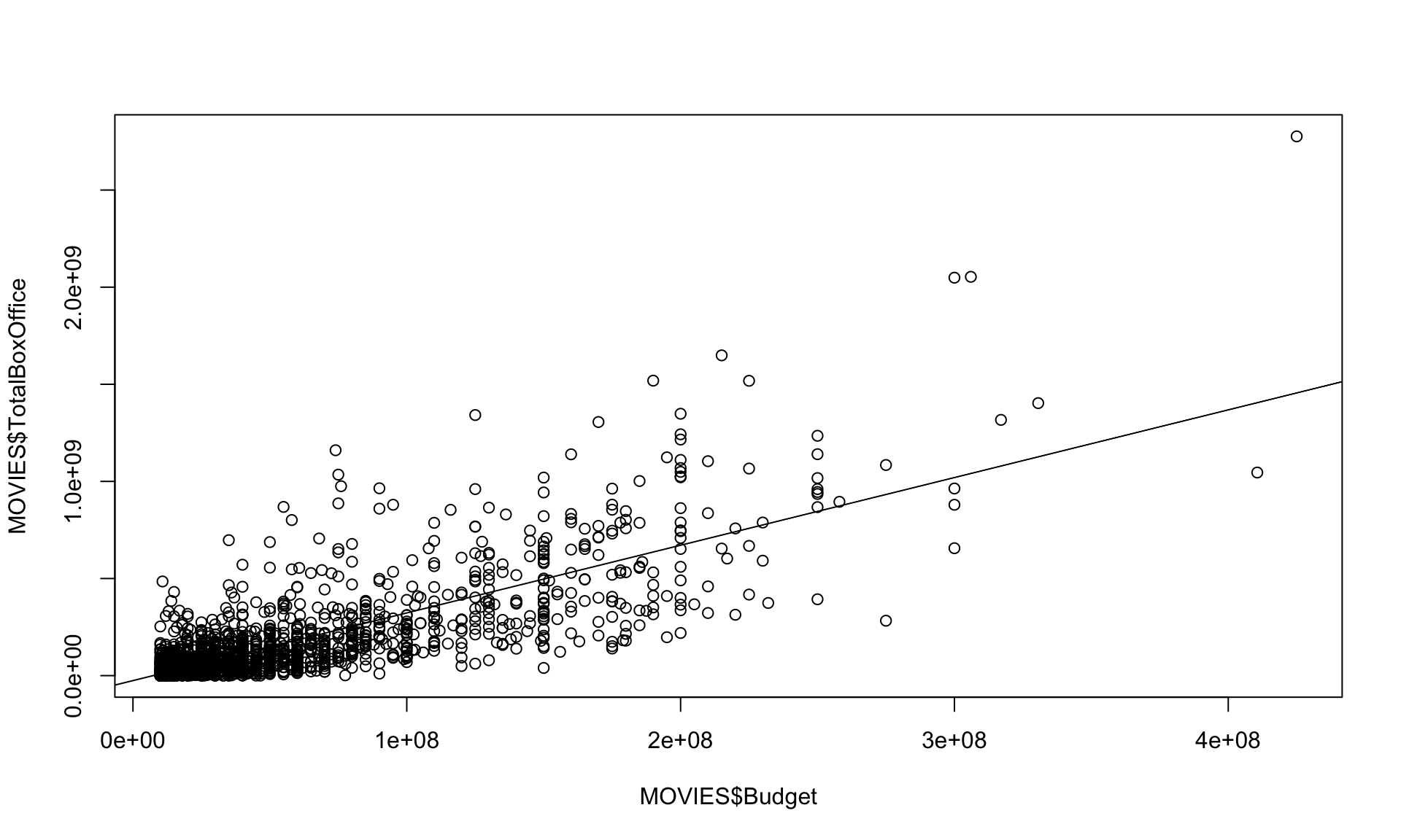
11.4.0.5 Session 6: Multiple Regression
Can we better predict Box Office revenue from other features?
##
## Call:
## lm(formula = TotalBoxOffice ~ Budget + Genre, data = MOVIES)
##
## Residuals:
##        Min         1Q     Median         3Q        Max
## -652147920  -58981135  -11395837   32951198 1316957185
##
## Coefficients:
##                 Estimate Std. Error t value Pr(>|t|)
## (Intercept)   -2.659e+07  9.551e+06  -2.784  0.00543 **
## Budget         3.496e+00  7.800e-02  44.825  < 2e-16 ***
## GenreComedy    3.717e+05  1.145e+07   0.032  0.97410
## GenreDrama    -3.065e+06  1.065e+07  -0.288  0.77348
## GenreHorror    3.150e+07  1.767e+07   1.783  0.07479 .
## GenreRomCom    1.278e+07  1.856e+07   0.688  0.49129
## GenreThriller -8.183e+06  1.245e+07  -0.657  0.51122
## ---
## Signif. codes:  0 '***' 0.001 '**' 0.01 '*' 0.05 '.' 0.1 ' ' 1
##
## Residual standard error: 1.51e+08 on 1761 degrees of freedom
## Multiple R-squared:  0.6142, Adjusted R-squared:  0.6128
## F-statistic: 467.2 on 6 and 1761 DF,  p-value: < 2.2e-16
11.4.0.6 Session 7: Variable Selection
What features should we include? (Note: we are using the package “olsrr” which should already be installed. If not, you will need to run the command install.packages(“olsrr”) for this to work.)
library(olsrr)
#MOVIES_LIMITED = select(MOVIES, c(Budget, Year ,Rating, Genre, Sequel, Runtime, TotalBoxOffice, ROI))
model3 = lm(TotalBoxOffice ~ Year + Sequel + Budget + Runtime, data = MOVIES)
forward = ols_step_forward_aic(model3)
print(forward)
##
##
## Stepwise Summary
## -------------------------------------------------------------------------------
## Step Variable AIC SBC SBIC R2 Adj. R2
## -------------------------------------------------------------------------------
## 0 Base Model 73289.914 73300.869 68270.458 0.00000 0.00000
## 1 Budget 71613.573 71630.006 66595.941 0.61298 0.61276
## 2 Sequel 71518.514 71540.425 66501.079 0.63366 0.63324
## 3 Runtime 71506.561 71533.949 66489.166 0.63654 0.63592
## 4 Year 71497.377 71530.243 66480.039 0.63883 0.63801
## -------------------------------------------------------------------------------
##
## Final Model Output
## ------------------
##
## Model Summary
## ----------------------------------------------------------------------------
## R 0.799 RMSE 145766157.098
## R-Squared 0.639 MSE 2.124777e+16
## Adj. R-Squared 0.638 Coef. Var 87.737
## Pred R-Squared 0.634 AIC 71497.377
## MAE 87074830.502 SBC 71530.243
## ----------------------------------------------------------------------------
## RMSE: Root Mean Square Error
## MSE: Mean Square Error
## MAE: Mean Absolute Error
## AIC: Akaike Information Criteria
## SBC: Schwarz Bayesian Criteria
##
## ANOVA
## ----------------------------------------------------------------------------
## Sum of
## Squares DF Mean Square F Sig.
## ----------------------------------------------------------------------------
## Regression 6.644574e+19 4 1.661143e+19 779.586 0.0000
## Residual 3.756606e+19 1763 2.130803e+16
## Total 1.040118e+20 1767
## ----------------------------------------------------------------------------
##
## Parameter Estimates
## ---------------------------------------------------------------------------------------------------------------
## model Beta Std. Error Std. Beta t Sig lower upper
## ---------------------------------------------------------------------------------------------------------------
## (Intercept) -7110977528.327 2095716362.344 -3.393 0.001 -1.122133e+10 -3.000627e+09
## Budget 3.140 0.072 0.705 43.495 0.000 2.998000e+00 3.281000e+00
## Sequel 101499059.397 10382257.364 0.152 9.776 0.000 8.113623e+07 1.218619e+08
## Runtime 681806.627 191265.714 0.054 3.565 0.000 3.066752e+05 1.056938e+06
## Year 3486905.352 1042486.908 0.048 3.345 0.001 1.442265e+06 5.531546e+06
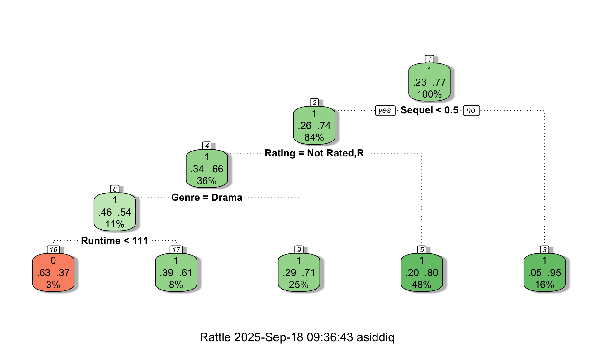
## ---------------------------------------------------------------------------------------------------------------11.4.0.7 Sessions 8 and 9: Logistic Regression and Classification Trees
Both of these sessions will focus on how to predict categorical variables, like whether or not a movie will generate a positive ROI. See below an example of a classification tree for answering this question. We are using two new packages for this example, this time “rpart” and “rattle”.
library(rpart)
library(rattle)
MOVIES$MadeMoney = ifelse(MOVIES$ROI>0,1,0)
RATED_MOVIES = subset(MOVIES, Rating != "")
tree = rpart(MadeMoney ~ Genre + Rating + Sequel + Runtime, data=RATED_MOVIES, method="class", cp = 0, maxdepth = 4)
fancyRpartPlot(tree,palettes=c("Reds", "Greens","Blues"))