Part 1 Modeling Uncertainty

Suppose you plan to book a ride from the Anderson complex to LAX airport next Friday at 12pm. How long will the drive be?

Of course, the precise travel time for your trip next week is uncertain, as a result of randomness in traffic conditions, weather, and countless other factors. This notion of uncertainty can be formalized using a random variable. In short, a random variable is a mathematical quantity that does not have a single, fixed value. Instead, random variables are defined by (1) a set of possible outcomes for the the variable (2) the probability (i.e., likelihood) of each outcome.

1.1 Probability and random variables

For example, suppose X is a random variable that describes the outcome of a coin toss. Here, the possible outcomes for \(X\) are \(\{Heads, Tails\}\), and the associated probabilities are \(P(X = Heads) = 0.5\) and \(P(X = Tails) = 0.5\). Similarly, we can define a random variable Y that describes the roll of a die, where the possible values are \(\{1,2,3,4,5,6\}\), and the probabilities are \(1/6\) for each outcome.

The outcome of a coin toss or die roll are two of the simplest possible examples of a random variable. They are both also examples of discrete random variables, which simply means the possible outcomes can be counted on (potentially many) hands. As you might have guessed, random variables can also be continuous, meaning the outcomes belong to a range of possible values. Examples of continuous random variables might be the temperature tomorrow in Fahrenheit or your credit card spending next month. In general, random variables are extremely flexible, and can be used to model virtually any kind of uncertainty.

A natural interpretation of probability is the long run relative frequency of an outcome after repeating an experiment independently a very large number of times. This is easy enough to conceptualize for rolling a die – the probability that we get a 4 in a single roll is equal to the the fraction of rolls that result in a 4 after 10,000 rolls. While this long run frequency interpretation is somewhat abstract for other probabilities (e.g. the likelihood of putting more than $1000 on your credit card next month), the same intuition applies.

1.2 The Normal distribution

As mentioned above, every random variable is defined by a set of possible outcomes and associated probabilities. For both discrete and continuous random variables, the correspondence between outcomes and probabilities is referred to as a probability distribution. The most well-known and useful probability distribution is arguably the Normal distribution, which you might know informally as the “bell curve”, and which will appear repeatedly throughout this course.

The Normal distribution is defined entirely by two parameters: the mean \(\mu\), which represents the average value, and standard deviation \(\sigma\), which represents variability around the mean. Returning to our travel time example, suppose the travel time from Anderson to LAX is a Normally-distributed random variable – let’s call it \(T\) – with a mean of \(\mu = 35\) minutes and a standard deviation of \(\sigma = 4.5\) minutes.

Note that \(T\) is a continuous random variable. One way of visualizing the distribution of continuous random variables is by looking at the density function:

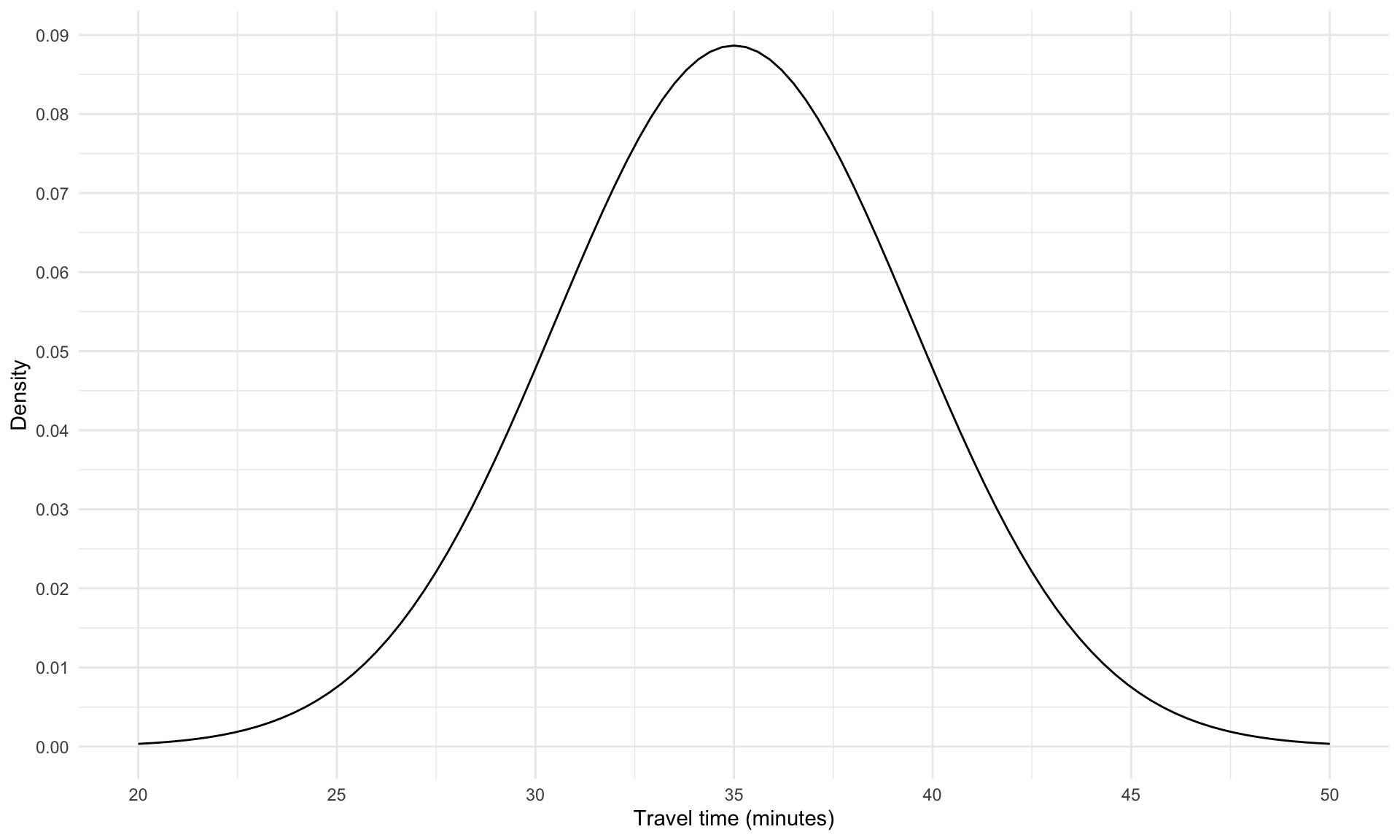
Informally, the plot above visualizes the likelihood that \(T\) takes on different values – travel times near the mean of \(30\) minutes are more likely than extremely travel times near 10 minutes or 50 minutes. However, the values on the vertical axis are not probabilities (they are “probability densities”, which we will not worry about in this course), so this plot is not particularly easy to interpret.

What is interpretable is a plot of the cumulative distribution function (CDF) of \(T\), which shows the probability that \(T\) is less than each of the values on the horizontal axis:

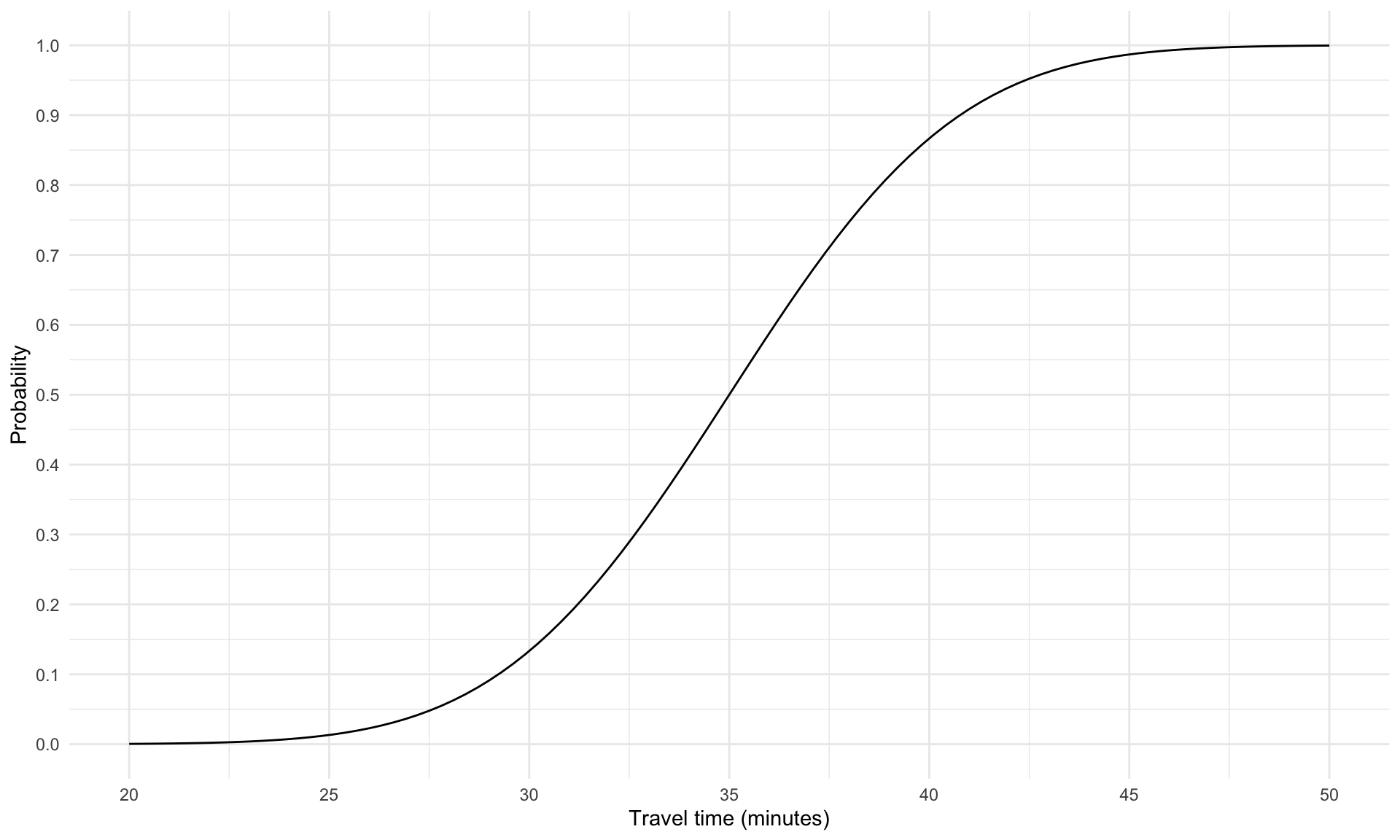
For example, the plot above tells us that the probability the trip takes less than 30 minutes is around 0.13 (\(P(T < 30) \approx 0.12\)), and the probability it takes less than 45 minutes is around 0.98 (\(P(T < 45) \approx 0.98\)). Note that the probability that \(T\) is less than the mean of 35 minutes is exactly 0.5, which is due to the symmetry of the Normal distribution – the trip is equally likely to take more than the average time as it is to take less.

1.3 Useful R commands

We will now look at three useful functions in R related to the normal distribution. First, let’s store the mean and standard deviation of the travel time variable \(T\):

mean = 35
sd = 4.5

Suppose we want to compute the probability that the trip takes less than 30 minutes – in other words, we want to read off the precise value of the CDF plot above at 30 minutes. We can do this in R using the pnorm() function:

pnorm(30, mean, sd, lower.tail = TRUE)

## [1] 0.1332603

In the line of code above, the option lower.tail = TRUE states that we want to determine \(P(T<30)\) – the probability that the trip takes less than 30 minutes. If we set lower.tail = FALSE, we get the probability that the trip takes more than 30 minutes (\(P(T>30)\)):

pnorm(30, mean, sd, lower.tail = FALSE)

## [1] 0.8667397

We have just used the pnorm() function to compute \(P(T < 30\) and \(P(T > 30)\), which we found to be 0.133 and 0.867, respectively. We can also ask the inverse question: Suppose we want to know what threshold value corresponds to the top 5% of travel times. Formally, this is equivalent to solving for \(x\) in \(P(T > x) = 0.05\). We can determine the answer by using the qnorm() function:

qnorm(0.05, mean, sd, lower.tail = FALSE)

## [1] 42.40184

A time of 42.4 is the threshold for the top 5% of travel times. Note that if we had set lower.tail = TRUE, we would get the threshold for the bottom 5% of travel times:

qnorm(0.05, mean, sd, lower.tail = TRUE)

## [1] 27.59816

We can also use qnorm() to identify the range of travel times that correspond to the middle 95% of the distribution, by checking the thresholds for the top and bottom 2.5%:

qnorm(0.025, mean, sd, lower.tail = TRUE)

## [1] 26.18016

qnorm(0.025, mean, sd, lower.tail = FALSE)

## [1] 43.81984

The results above imply that 95% of trips take between 26.2 and 43.8 minutes.

The last function we will look at is rnorm(), which allows us to randomly “draw” one or more values from a Normal distribution. In the code below, count stores the number of values we we want to draw from the distribution. Recall that mean and sd are storing the mean and standard deviation of the travel time random variable \(T\). If we want to randomly generate one value, we can then use

count = 1
rnorm(count,mean,sd)

## [1] 38.26217

We can randomly generate 10 values by updating the count variable and calling rnorm() again:

count = 10
rnorm(count,mean,sd)

##  [1] 30.81580 33.71510 39.53986 31.50431 39.02663 42.65759 34.39838 41.41285
##  [9] 38.36965 35.35811

The rnorm() command is especially helpful for building Monte Carlo simulation models, which is the focus of the next section.