Part 2 Monte Carlo Simulation
Monte Carlo simulation refers to the use of computational methods to model the behavior of a random process. For example, suppose we wanted to know the probability that the sum of two dice adds up to exactly 7. We can figure this out with some effort, because we know there are 36 possible combinations of two dice, and six of them add up to 7 (1+6, 2+5, 3+4, 4+3, 5+2, and 6+1). So the probability that the sum of two dice adds up to exactly 7 is 6/36, or 1/6.
But what if we asked a more complicated question: What is the probability that the sum of five dice adds up to at least 20? Instead of trying to figure out the answer using (potentially difficult) math, we can get a reasonable estimate by just rolling five dice 100 times, and then counting the number of rolls in which the sum is at least 20. Even better, we don’t need real dice, because we can just write R code that “rolls” dice by generating random numbers between 1 and 6. And instead of rolling the dice 100 times, we can just as easily do it 1,000 or 10,000 times to get a more accurate estimate, due to the law of large numbers and the “long run frequency” interpretation of probability.
This is the general idea behind Monte Carlo simulation – we use a computer to simulate a complex, random process, which allows us to estimate the probability distribution of the possible outcomes.
In practice, there are numerous examples of Monte Carlo simulation (which we will just call “simulation” from now on):
- In finance, simulation is used to account for uncertainty when creating forecasts of portfolio returns (https://www.portfoliovisualizer.com/monte-carlo-simulation).
- In election modeling, simulation is used to model possible outcomes of an election (https://projects.fivethirtyeight.com/trump-biden-election-map/),
- Simulation models have also been used to model the spread of COVID over time (https://covid19.healthdata.org/).
This tutorial will cover a simple but fundamental example of simulation: drawing random samples from a Normal distribution. We will use the purrr package, which contains the replicate() function that is useful for simulation.
2.1 Example: Revenue management
We will explore how to simulate from a Normal distribution using the following hypothetical example. Suppose Sidecar Donuts in Santa Monica sells Old Fashion donuts for $3.50 each. Based on historical data, Sidecar has determined that the daily demand for old-fashioned donuts is normally distributed with \(\mu = 60\) and \(\sigma = 20\). Suppose each donut costs $1.00 to make, and Sidecar makes 90 donuts per day. Further,
- If the demand for donuts exceeds 90, then Sidecar sells all 90 and cannot serve the remaining customers.
- If the demand for donuts is less than 90, then the leftover donuts are discarded at the end of the day.
Let’s now consider how we can set up a simulation to analyze Sidecar’s business. In particular, we will consider the following four questions:
- What does the distribution of Sidecar’s daily demand look like?
- What does the distribution of Sidecar’s daily quantity sold look like?
- What does the forecast of Sidecar’s weekly profit look like, and what is the weekly expected (i.e. average case) profit?
- What is the impact of Sidecar’s donut production on daily expected profit?
Each question builds on the one before. Let’s consider them one at a time.
2.2 Simulating daily demand
The only source of randomness in this problem is the daily demand for donuts, which we know is normally distributed with \(\mu = 60\) and \(\sigma = 20\). For convenience, let’s store these values:
First, let’s visualize Sidecar’s daily demand for donuts. We can run 20 simulations using the following code:
Let’s unpack what is going on in the code above:
The variable
simstores the number of times we want to repeat the simulation.The
rnorm()function draws numbers from a Normal distribution. Going from left to right, the first entry inrnorm()is the number of values we want to pull from the Normal distribution, the second is the mean of the Normal distribution, and the third is the standard deviation of the Normal distribution.Calling the
rnorm()function a single time represents one draw from the Normal distribution (one “roll of the dice”). To see the distribution of demand, we callrnorm()20 times usingreplicate(). The end result is thatdaily_demandstores 20 draws from the specified Normal distribution.
We can now visualize the distribution of demand using a histogram:
library(MetBrewer)
cols = met.brewer("Monet")
hist(daily_demand, main="Daily Demand", xlab="Demand", ylab="Frequency", col=cols[8])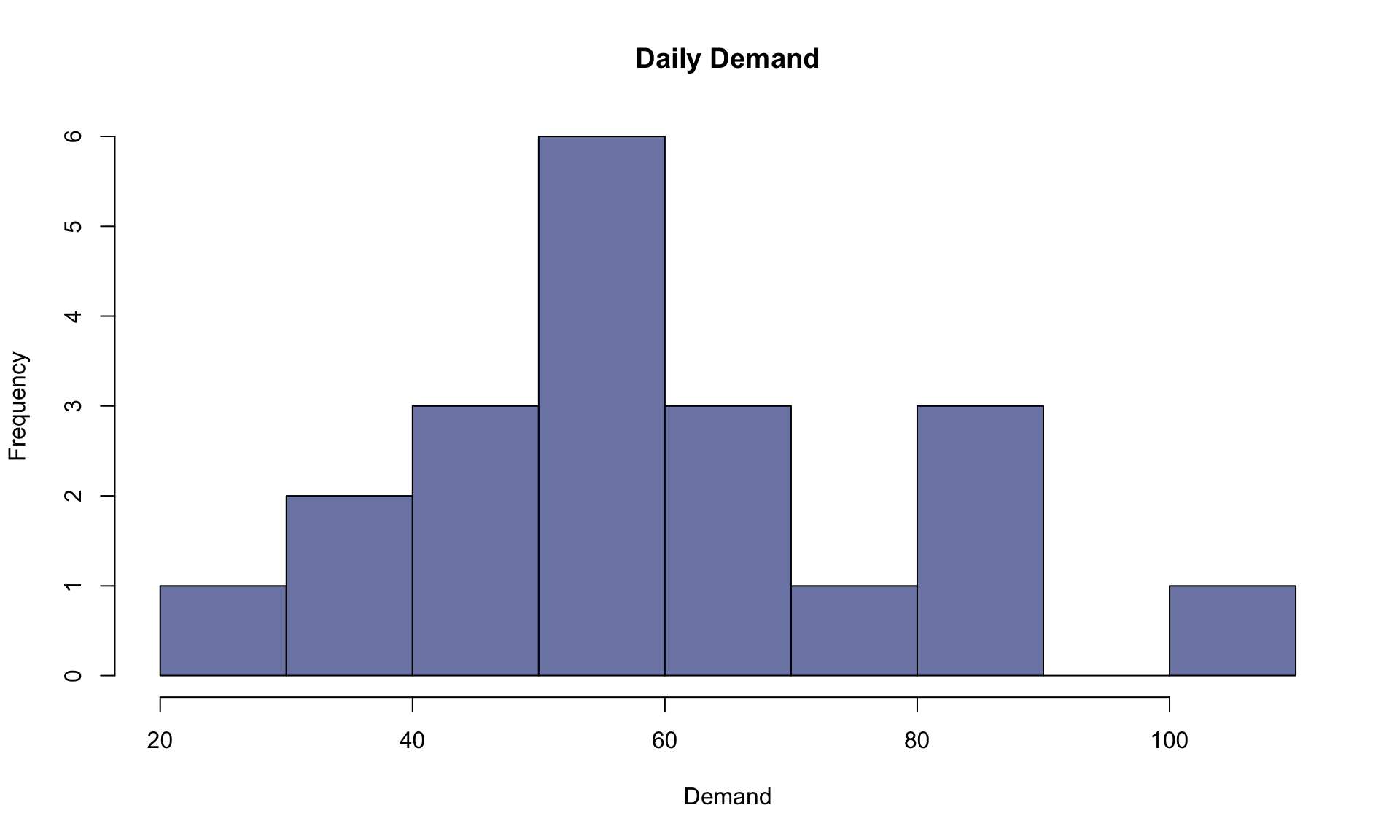
The histogram above shows the range of possible demand values obtained by the 20 simulation runs. What if used 10,000 runs instead of 20?
sims = 10000
daily_demand <- replicate(n = sims, rnorm(1,mean,sd), simplify = TRUE)
hist(daily_demand, main="Daily Demand", xlab="Demand", ylab="Frequency", col=cols[8], xlim=c(0,120))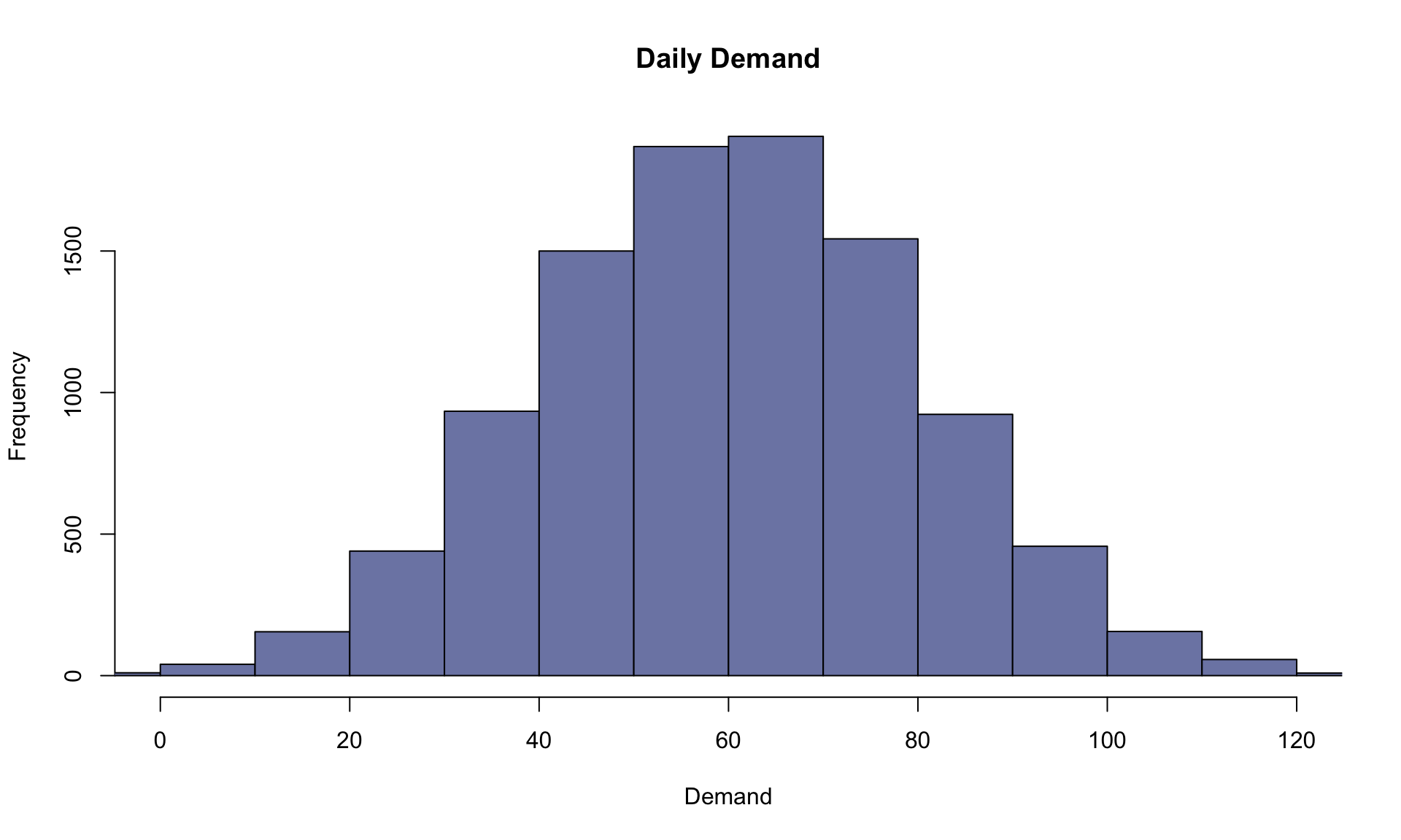
We can see that the graph above after using 10,000 runs looks much more similar to the familiar “bell curve” shape of the Normal distribution. This is the law of large numbers in action: the larger the number of simulation runs, the more accurately the results reflect the underlying probability distribution.
2.3 Simulating daily quantity sold
Let’s now visualize the daily quantity of donuts sold. We can do this in a similar way as above, except now we need to keep track of the fact that Sidecar can’t sell more donuts than it makes, which is 90. To simulate the number of donuts sold, we will use the pmin() function to take the smaller number between the (random) demand and 90:
sims = 10000
count = 90
daily_quantity <- replicate(n = sims, pmin(rnorm(1,mean,sd),count), simplify = TRUE)
In the code above, we store the number of donuts available in the variable count. Next, creating a histogram allows us to visualize the range of possible donut sales:
hist(daily_quantity, main="Daily Quantity Sold", xlab="Quantity", ylab="Frequency", col=cols[5],xlim=c(0,120))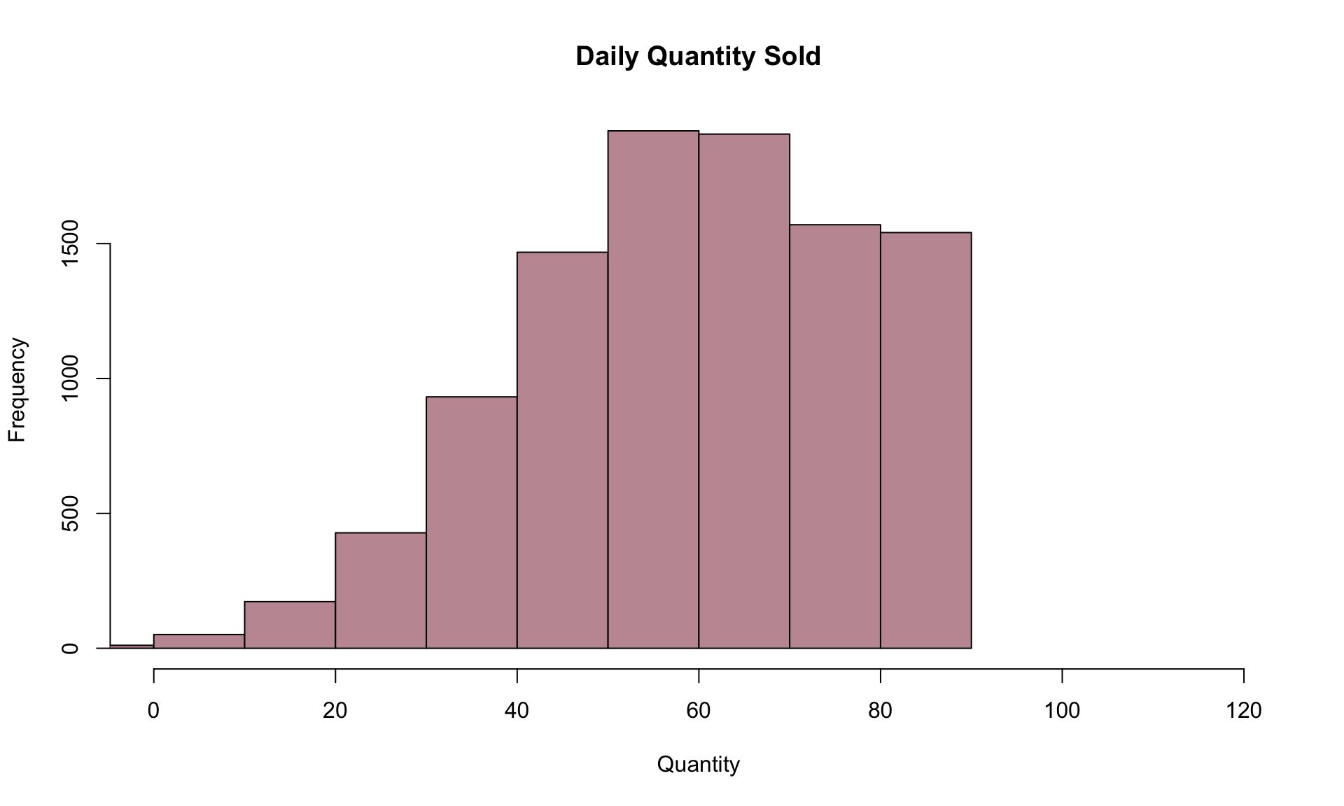
The distribution of daily quantity sold is very similar to the distribution of daily demand in 2.1, but is “cut off” at 90. If we now want to estimate the expected value of the daily quantity, we can take the average over all 10,000 simulation runs:
## [1] 59.34327Note that the expected quantity sold is slightly lower than the mean demand of 60.
2.4 Simulating weekly profit
Let’s now forecast Sidecar’s weekly profit. We now need to keep track of two more parameters: the price of and production cost of one donut:
The weekly profit is given by total revenue (price x quantity sold) minus total cost (cost x quantity produced) over a 7-day period. We can simulate weekly profit 100 times using the following code:
set.seed(0)
sims = 100
days = 7
daily_profit <- replicate(n = sims, price*pmin(rnorm(days,mean,sd),count)-cost*count, simplify = TRUE)
There are two changes between the code above and the block from 2.2:
- We now simulate a week of sales instead of one day (look for the where `days’ variable shows up in the code),
- we now multiply the quantity sold by
price, to get revenue, and - we subtract off the total weekly cost (
cost*count) to get profit.
The variable `weekly_profit’ is a table with 7 rows and 100 columns, with each column representing a 7-day simulation of sales. Next, with a bit of data manipulation, we can determine the cumulative profit over the 7-day period in each simulation run, and plot the resulting forecasts:
cumulative_profit <- apply(daily_profit,2,cumsum)
avg_cumulative_profit <- rowMeans(cumulative_profit)
plot(0, 0, type = 'n', xlim = c(1, days), ylim = c(0, 1000), xlab = 'Day', ylab = 'Cumulative profit')
for (i in 1:sims) lines(1:days, cumulative_profit[,i], col = alpha("grey", 0.2), lwd = 1)
lines(1:days, avg_cumulative_profit, col = alpha(cols[1], 1), lwd = 2)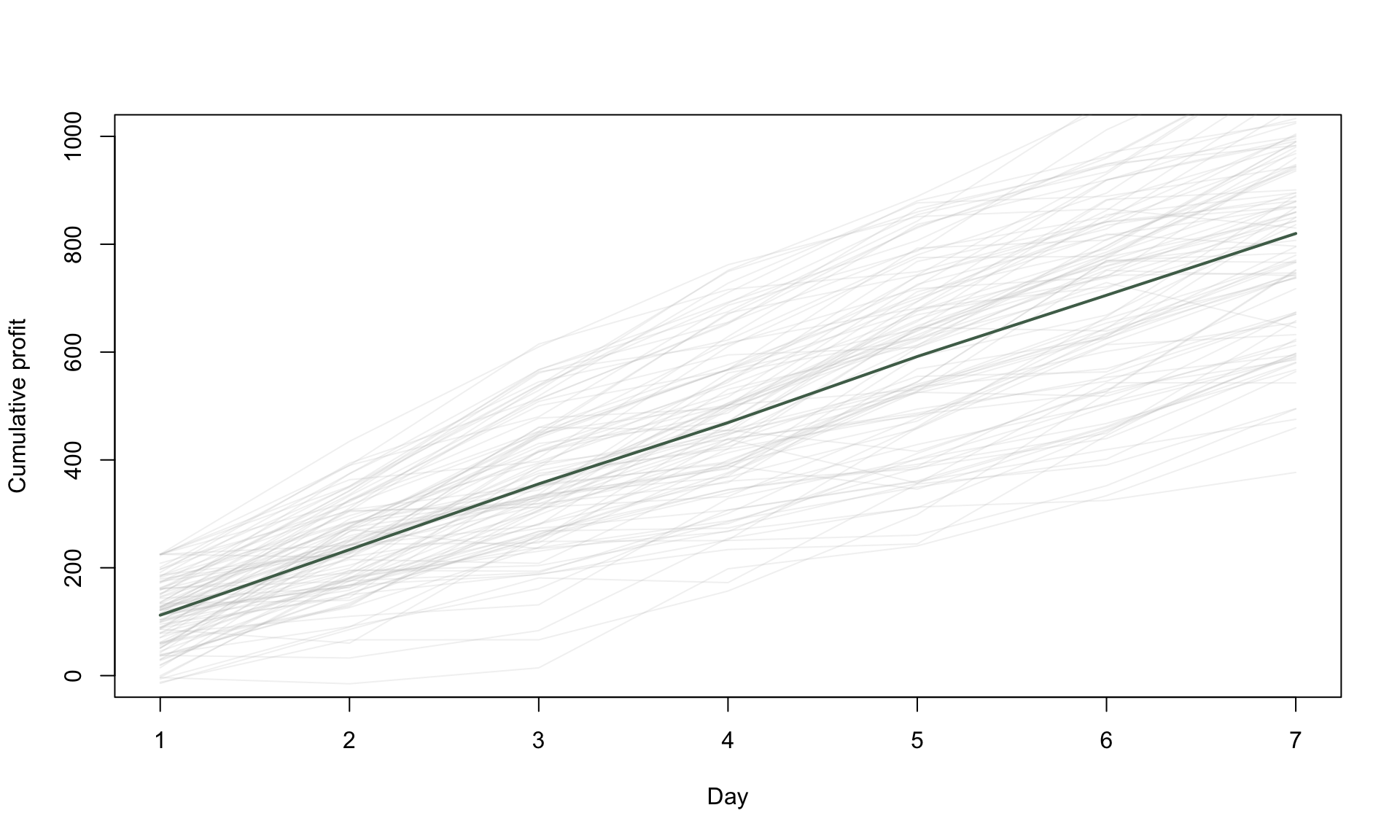
Each gray line in the plot above represents one possible scenario for the cumulative profit over a 7-day period, and corresponds to one simulation run. We can think of the collection of gray lines as describing the range of possible scenarios. The green line is the average of all of 100 scenarios. If we now repeat it for 10,000 simulation runs, we get a more general idea of the overall forecast:
set.seed(0)
sims = 10000
days = 7
daily_profit <- replicate(n = sims, price*pmin(rnorm(days,mean,sd),count)-cost*count, simplify = TRUE)
cumulative_profit <- apply(daily_profit,2,cumsum)
avg_cumulative_profit <- rowMeans(cumulative_profit)

plot(0, 0, type = 'n', xlim = c(1, days), ylim = c(0, 1000), xlab = 'Day', ylab = 'Cumulative profit')
for (i in 1:sims) lines(1:days, cumulative_profit[,i], col = alpha('grey', 0.03), lwd = 0.5)
lines(1:days, avg_cumulative_profit, col = alpha(cols[1], 1), lwd = 2)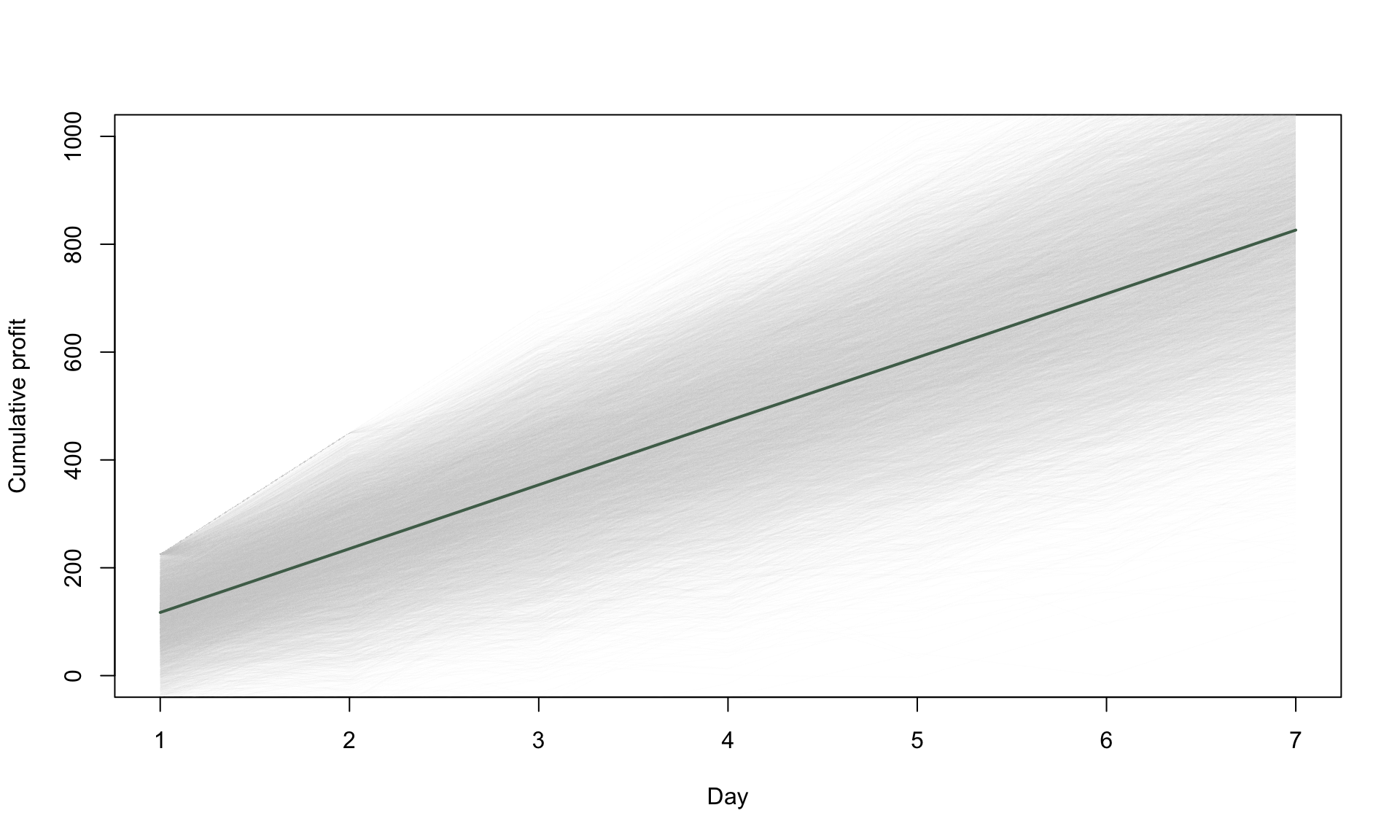
We can also create a histogram of total profit after a 7-day period by looking at the 7th row of the cumulative_profit variable:
weekly_profit = cumulative_profit[7,]
hist(weekly_profit, main="Weekly Profit", xlab="Profit", ylab="Frequency", col=cols[1])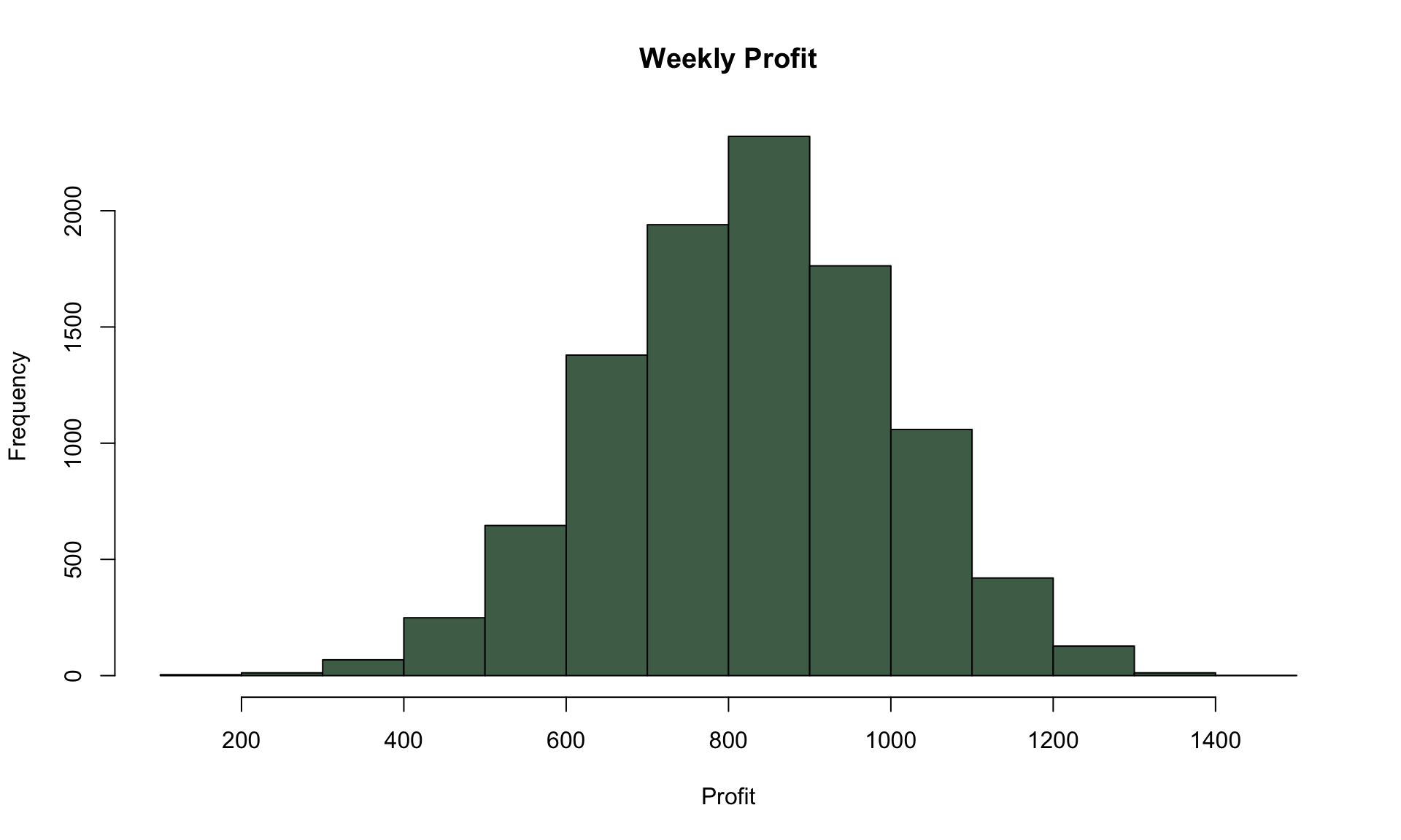
2.5 Assessing risk
Because Monte Carlo simulation provides a distribution of possible outcomes, it is commonly used for risk analysis. For example, suppose we wanted to fill in the blank in the following statement:
The probability that weekly profit is below $600 is ____.
We can determine what goes in the blank using the ecdf() function (which refers to empirical cumulative distribution function):
## [1] 0.0979The ecdf() function above looks at all 10,000 simulated profit values after the 7th day of operation, and calculates the fraction of simulation runs that produced a weekly profit of below $600. Based on the law of large numbers, we interpret this fraction of simulation runs as the probability that weekly profit is below $600.
Alternatively, we can flip the question to try to fill in the blank below:
The probability that weekly profit is below ____ is 0.2.
We can determine what goes in the blank by using the quantile() function:
##      20%
## 679.6135
The results tell us that 10% of simulation runs, the weekly profit will be below $678. Similarly, we can use the quantile() function to determine a 95% interval for the weekly profit:
##     2.5%
## 478.4233## 97.5%
## 1163.019In 95% of simulations, the weekly profit is between $476 and $1154.
2.6 Profit optimization
Let’s now consider how donut production affects daily profit. The code below re-runs the simulation for different values of the count variable, which represents the number of donuts made daily. Then the exp_profit variable stores the estimated daily profit, which is calculated as the average over all 10,000 simulations.
sims = 10000

exp_profit <- matrix(nrow=10, ncol=1)
donuts_made <- matrix(nrow=10, ncol=1)

for(i in 1:10){
  count = i*10
profit <- replicate(n = sims, price*pmin(rnorm(1,mean,sd),count)-cost*count, simplify = TRUE)
exp_profit[i] <- mean(profit)
donuts_made[i] <- count
}
Next, we can visualize the impact of the number of donuts made on daily profit:
plot(donuts_made, exp_profit, pch = 16, col = cols[1], type = 'b', xlab = 'Donuts made daily', ylab = 'Expected daily profit')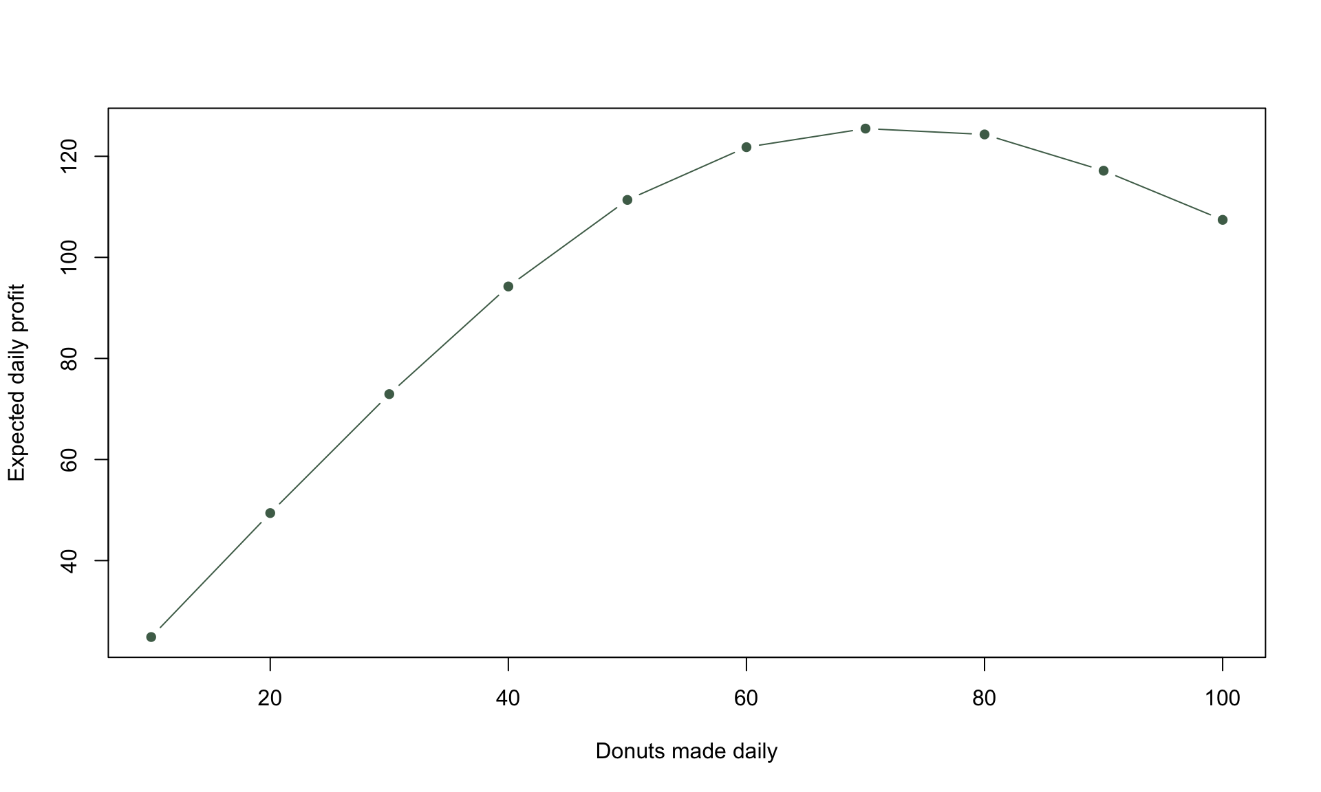
Based on the plot above, daily profit appears to be maximized at a daily production of 70, and not the current value of 90. We can get the exact values by printing exp_profit and donuts_made:
##       [,1]
##  [1,]   10
##  [2,]   20
##  [3,]   30
##  [4,]   40
##  [5,]   50
##  [6,]   60
##  [7,]   70
##  [8,]   80
##  [9,]   90
## [10,] 100## [,1]
## [1,] 24.87329
## [2,] 49.40139
## [3,] 72.93989
## [4,] 94.24131
## [5,] 111.36783
## [6,] 121.80570
## [7,] 125.48601
## [8,] 124.32532
## [9,] 117.14952
## [10,] 107.42612Based on the printouts above, we see that producing 70 donuts leads to a daily profit of $125.4, whereas the current practice of making 90 donuts per day gives $117.5 – a profit lift of about 7%.
Monte Carlo simulation is a useful method for creating predictions in the face of uncertainty or randomness. Here we demonstrated a simple simulation model based on randomly generating values from a Normal distribution. The general principles discussed above can be extended to many other distributions (discrete or continuous), as well as multiple sources of randomness.