Part 8 Variable Selection
Here we discuss a few different approaches to variable selection in R.
8.1 Data: Airbnb listings
We will use the airbnb_small.csv dataset, which contains information on 50 Airbnb listings in Florence, Italy from 2021. There are 24 variables for each listing, which includes information on hosts, location, price, property details, and reviews. Our goal will be to build a model that predicts the price of the Airbnb property from the remaining variables.
Two useful packages are olsrr and glmnet, which have convenient built-in methods for variable selection. Let’s start by loading these packages, setting our working directory, and reading in the file:
8.2 Stepwise regression
When we have a large number of potential variables to choose from for regression, simply throwing all of them into the model might make the model too complex. High model complexity has two drawbacks:
- it makes interpreting and explaining the model to others more complicated, and
- it risks overfitting the model to data, which can erode predictive performance.
One way of controlling model complexity in linear regression is called stepwise regression.
The key to stepwise regression is a performance metric called the Akaike information criterion (AIC). The AIC of a regression model measures how well the model balances complexity (i.e., the number of variables included in the regression) and goodness-of-fit (i.e., how well the chosen set of variables fit the data). In general, a regression model with a lower AIC is viewed as achieving a “better” balance between complexity and goodness-of-fit. The AIC is therefore widely used as a guide for finding a small number of variables with high explanatory power.
8.2.1 Stepwise regression with forward selection
One approach to stepwise regression is called forward selection. The general idea is that we start with a “blank” model, add whichever variable improves (i.e., decreases) the AIC the most, and repeat until the AIC can’t be improved any further.
Building a stepwise model in R is similar to building a standard linear regression model, but takes one extra step. Using the airbnb.csv First we run a regular linear regression using lm(), with Price as the dependent variable:
As a benchmark, let’s look at the results of the full linear regression model:
##
## Call:
## lm(formula = Price ~ ., data = airbnb)
##
## Residuals:
## Min 1Q Median 3Q Max
## -56.613 -10.105 -0.221 12.286 49.415
##
## Coefficients:
## Estimate Std. Error t value Pr(>|t|)
## (Intercept) 13516.3486 56832.9384 0.238 0.8144
## HostResponseTimewithin a day -475.6676 213.3597 -2.229 0.0374 *
## HostResponseTimewithin a few hours -493.5318 203.8891 -2.421 0.0251 *
## HostResponseTimewithin an hour -455.0459 207.1368 -2.197 0.0400 *
## HostResponseRate 390.4220 220.2179 1.773 0.0915 .
## HostAcceptRate 31.5768 39.6043 0.797 0.4346
## Superhost -7.6700 13.5703 -0.565 0.5782
## HostListings 0.7634 0.2810 2.716 0.0133 *
## NeighbourhoodCentro Storico 4.9871 37.1483 0.134 0.8945
## NeighbourhoodGavinana Galluzzo -186.4095 1012.4128 -0.184 0.8558
## NeighbourhoodIsolotto Legnaia -103.9420 83.4928 -1.245 0.2276
## NeighbourhoodRifredi -28.8847 43.0517 -0.671 0.5099
## Latitude 60.4395 1238.8568 0.049 0.9616
## Longitude -1464.6477 1062.1974 -1.379 0.1832
## RoomTypeHotel room 50.2613 33.7877 1.488 0.1525
## RoomTypePrivate room -5.8018 24.4563 -0.237 0.8149
## Accomodates 12.1546 6.7288 1.806 0.0859 .
## Bathrooms -19.7126 13.0087 -1.515 0.1453
## Bedrooms 29.1729 15.6235 1.867 0.0766 .
## Beds -2.6974 10.8947 -0.248 0.8070
## MinNights 1.0589 2.6414 0.401 0.6928
## AvgRating -51.2645 75.8444 -0.676 0.5068
## RatingAccuracy -31.8468 35.4207 -0.899 0.3793
## RatingClean 11.9607 63.9980 0.187 0.8536
## RatingCheckIn 22.1832 88.4108 0.251 0.8044
## RatingCommunication 85.7820 75.2299 1.140 0.2676
## RatingLocation -55.6150 43.7572 -1.271 0.2183
## RatingValue 102.3121 55.8141 1.833 0.0817 .
## InstantBook -17.9653 16.8469 -1.066 0.2990
## ReviewsPerMonth -4.2126 6.0649 -0.695 0.4953
## ---
## Signif. codes: 0 '***' 0.001 '**' 0.01 '*' 0.05 '.' 0.1 ' ' 1
##
## Residual standard error: 32.55 on 20 degrees of freedom
## Multiple R-squared: 0.8794, Adjusted R-squared: 0.7045
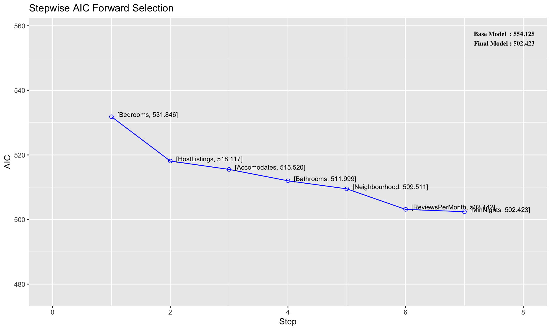
## F-statistic: 5.028 on 29 and 20 DF, p-value: 0.0002066Then we send our stored model to the ols_step_forward_aic() function (which comes from the olsrr package), which will automatically perform the stepwise regression:
To see the full set of results and the variables that are added at each step, we simply use print():
##
##
##                                 Stepwise Summary
## ------------------------------------------------------------------------------
## Step    Variable             AIC        SBC       SBIC        R2       Adj. R2
## ------------------------------------------------------------------------------
##  0      Base Model         554.125    557.949    409.858    0.00000    0.00000
##  1      Bedrooms           531.846    537.583    387.393    0.38465    0.37183
##  2      HostListings       518.117    525.765    374.034    0.55074    0.53163
##  3      Accomodates        515.520    525.080    371.373    0.59021    0.56348
##  4      Bathrooms          511.999    523.471    368.259    0.63305    0.60043
##  5      Neighbourhood      509.511    528.631    361.779    0.70248    0.64443
##  6      ReviewsPerMonth    503.142    524.174    357.944    0.74834    0.69171
##  7      MinNights          502.423    525.368    358.631    0.76165    0.70054
## ------------------------------------------------------------------------------
##
## Final Model Output
## ------------------
##
##                          Model Summary
## ----------------------------------------------------------------
## R                        0.873       RMSE                28.942
## R-Squared                0.762       MSE                837.642
## Adj. R-Squared           0.701       Coef. Var           36.115
## Pred R-Squared            -Inf       AIC                502.423
## MAE                     18.964       SBC                525.368
## ----------------------------------------------------------------
##  RMSE: Root Mean Square Error
##  MSE: Mean Square Error
##  MAE: Mean Absolute Error
##  AIC: Akaike Information Criteria
##  SBC: Schwarz Bayesian Criteria
##
##                                 ANOVA
## ----------------------------------------------------------------------
##                   Sum of
##                  Squares        DF    Mean Square      F         Sig.
## ----------------------------------------------------------------------
## Regression    133837.507        10      13383.751    12.463    0.0000
## Residual       41882.113        39       1073.900
## Total         175719.620        49
## ----------------------------------------------------------------------
##
##                                               Parameter Estimates
## ----------------------------------------------------------------------------------------------------------------
##                          model       Beta    Std. Error    Std. Beta      t        Sig        lower       upper
## ----------------------------------------------------------------------------------------------------------------
##                    (Intercept)     42.093        24.588                  1.712    0.095      -7.642      91.827
##                       Bedrooms     22.657        10.726        0.288     2.112    0.041       0.961      44.352
##                   HostListings      0.495         0.129        0.314     3.832    0.000       0.234       0.756
##                    Accomodates     11.967         4.473        0.384     2.676    0.011       2.920      21.014
##                      Bathrooms    -31.706         9.829       -0.280    -3.226    0.003     -51.587     -11.826
##    NeighbourhoodCentro Storico     23.629        16.649        0.179     1.419    0.164     -10.047      57.306
## NeighbourhoodGavinana Galluzzo    832.596       512.196        1.966     1.626    0.112    -203.419    1868.610
##  NeighbourhoodIsolotto Legnaia    -39.923        29.538       -0.132    -1.352    0.184     -99.668      19.823
##           NeighbourhoodRifredi     -8.569        22.240       -0.043    -0.385    0.702     -53.554      36.415
##                ReviewsPerMonth    -10.633         3.577       -0.261    -2.973    0.005     -17.867      -3.398
##                      MinNights     -2.117         1.434       -1.816    -1.476    0.148      -5.018       0.784
## ----------------------------------------------------------------------------------------------------------------
The output above tells us that the first variable added to the model is Bedrooms, and that this one-variable achieves \(AIC = 532\) and \(R^2 = 0.385\). Then a two-variable linear model with both Bedrooms and HostListings achieves \(AIC = 518\) and \(R^2 = 0.551\), and so on. Note that the output above lists only 7 out of the 23 possible independent variables we could have used.
Next, visualizing AIC is straightforward using plot():
8.2.2 Stepwise regression with backward elimination
Another way of performing stepwise regression is backward elimination, which is conceptually similar to forward selection. In backward elimination, we start with a “full” model that contains all possible variables, and then we identify the variable whose removal from the model improves the AIC the most, and repeat until the AIC cannot be improved further.
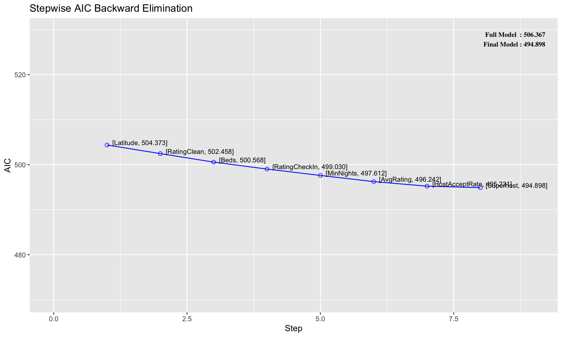
The R code for backward elimination is similar: first we run the full linear regression model using lm(), and then we use ols_step_backward_aic():
Like in forward selection, we can print the model to see the result of each step:
##
##
##                                Stepwise Summary
## -----------------------------------------------------------------------------
## Step    Variable            AIC        SBC       SBIC        R2       Adj. R2
## -----------------------------------------------------------------------------
##  0      Full Model        506.367    565.639    419.973    0.87939    0.70450
##  1      Latitude          504.373    561.733    410.189    0.87937    0.71854
##  2      RatingClean       502.458    557.907    401.324    0.87917    0.73087
##  3      Beds              500.568    554.105    393.223    0.87890    0.74200
##  4      RatingCheckIn     499.030    550.655    386.123    0.87777    0.75046
##  5      MinNights         497.612    547.324    379.718    0.87635    0.75764
##  6      AvgRating         496.242    544.043    373.875    0.87478    0.76400
##  7      HostAcceptRate    495.231    541.119    368.848    0.87228    0.76821
##  8      Superhost         494.898    538.875    364.913    0.86794    0.76890
## -----------------------------------------------------------------------------
##
## Final Model Output
## ------------------
##
##                          Model Summary
## ----------------------------------------------------------------
## R                        0.932       RMSE                21.543
## R-Squared                0.868       MSE                464.097
## Adj. R-Squared           0.769       Coef. Var           31.726
## Pred R-Squared            -Inf       AIC                494.898
## MAE                     15.842       SBC                538.875
## ----------------------------------------------------------------
##  RMSE: Root Mean Square Error
##  MSE: Mean Square Error
##  MAE: Mean Absolute Error
##  AIC: Akaike Information Criteria
##  SBC: Schwarz Bayesian Criteria
##
##                                 ANOVA
## ---------------------------------------------------------------------
##                   Sum of
##                  Squares        DF    Mean Square      F        Sig.
## ---------------------------------------------------------------------
## Regression    152514.786        21       7262.609    8.763    0.0000
## Residual       23204.834        28        828.744
## Total         175719.620        49
## ---------------------------------------------------------------------
##
##                                                   Parameter Estimates
## ------------------------------------------------------------------------------------------------------------------------
##                              model         Beta    Std. Error    Std. Beta      t        Sig         lower        upper
## ------------------------------------------------------------------------------------------------------------------------
##                        (Intercept)    16248.212      7816.138                  2.079    0.047      237.579    32258.845
##       HostResponseTimewithin a day     -478.262       166.018       -1.581    -2.881    0.008     -818.334     -138.190
## HostResponseTimewithin a few hours     -503.945       160.664       -2.950    -3.137    0.004     -833.050     -174.840
##     HostResponseTimewithin an hour     -465.391       162.138       -3.353    -2.870    0.008     -797.515     -133.267
##                   HostResponseRate      428.393       167.135        1.497     2.563    0.016       86.033      770.753
##                       HostListings        0.860         0.166        0.546     5.196    0.000        0.521        1.199
##        NeighbourhoodCentro Storico       -1.922        24.825       -0.015    -0.077    0.939      -52.773       48.930
##     NeighbourhoodGavinana Galluzzo      239.102        93.577        0.565     2.555    0.016       47.418      430.787
##      NeighbourhoodIsolotto Legnaia     -114.779        61.572       -0.379    -1.864    0.073     -240.903       11.345
##               NeighbourhoodRifredi      -34.656        31.113       -0.175    -1.114    0.275      -98.389       29.076
##                          Longitude    -1467.268       693.156       -0.385    -2.117    0.043    -2887.134      -47.403
##                 RoomTypeHotel room       48.958        24.015        0.162     2.039    0.051       -0.234       98.150
##               RoomTypePrivate room        1.278        17.652        0.006     0.072    0.943      -34.880       37.437
##                        Accomodates       11.259         4.644        0.362     2.424    0.022        1.746       20.772
##                          Bathrooms      -25.234         8.778       -0.223    -2.875    0.008      -43.215       -7.253
##                           Bedrooms       28.714        10.491        0.365     2.737    0.011        7.224       50.205
##                     RatingAccuracy      -33.234        26.964       -0.384    -1.233    0.228      -88.467       21.998
##                RatingCommunication       67.552        33.123        0.630     2.039    0.051       -0.298      135.401
##                     RatingLocation      -39.816        32.630       -0.439    -1.220    0.233     -106.655       27.024
##                        RatingValue       80.270        32.846        0.906     2.444    0.021       12.988      147.552
##                        InstantBook      -18.073        11.221       -0.148    -1.611    0.118      -41.058        4.912
##                    ReviewsPerMonth       -5.342         4.291       -0.131    -1.245    0.223      -14.133        3.448
## ------------------------------------------------------------------------------------------------------------------------
In the table above, we can see the names of 8 variables that are eliminated from the model. In this example, the final model from backward elimination achieves \(AIC = 495\) and \(R^2 = 0.868\). Note that backward elimination arrives at a different final model than forward selection in this case.
Similar to before, we can use plot() to visualize the result of the stepwise regression based on backward elimination:
8.3 LASSO regression
Another popular method for variable selection is LASSO regression. In general, LASSO is used when dealing with a huge number of potential variables, in which case stepwise regression can be very slow. (There are other differences that we won’t get into here).
8.3.1 Building a LASSO regression model
LASSO regression can be done in R using the glmnet() function. In order to apply it to the Airbnb data, we first need to do a little bit of data manipulation. In particular, we need to manually convert the columns with character strings (i.e., words) into R factors, and then convert the factors into 0 or 1 binary variables using “one-hot” encoding. The code below does this:
airbnb$HostResponseTime <- as.factor(airbnb$HostResponseTime)
airbnb$RoomType <- as.factor(airbnb$RoomType)
airbnb$Neighbourhood <- as.factor(airbnb$Neighbourhood)

airbnbone <- one_hot(as.data.table(airbnb))
If we take a look at the new data frame, we can see that it now has 34 columns, due to the conversion of the factor variables into 0-1 dummy variables. (It is commented out below to simplify HTML output, but you can run it in R Markdown to preview the new data frame).
Next, we need to split the dataframe into independent and dependent variables. (We have to do this because the glmnet() function we will use for LASSO regression expects the data to be in a different format from the stepwise regression functions we used above). For simplicity we will use x and y to denote the independent and dependent variables, respectively:
x <-as.matrix(subset(airbnbone, select=-c(Price)))
y <-as.matrix(subset(airbnbone, select=c(Price)))
Now that the data is formatted, we can call glmnet() to run a lasso regression:
Printing the results displays the number of variables selected at each value of \(\lambda\) (Df = degrees of freedom):
##
## Call:  glmnet(x = x, y = y)
##
##    Df  %Dev Lambda
## 1   0  0.00 36.770
## 2   2  7.19 33.500
## 3   2 13.22 30.520
## 4   2 18.24 27.810
## 5   3 23.99 25.340
## 6   3 29.94 23.090
## 7   3 34.88 21.040
## 8   3 38.98 19.170
## 9   3 42.38 17.470
## 10  3 45.21 15.920
## 11  3 47.55 14.500
## 12  3 49.50 13.210
## 13  4 51.49 12.040
## 14  5 53.80 10.970
## 15  7 56.68  9.995
## 16  7 59.60  9.108
## 17  8 62.07  8.298
## 18  9 64.32  7.561
## 19  9 66.40  6.889
## 20  9 68.13  6.277
## 21  9 69.57  5.720
## 22  9 70.76  5.212
## 23 10 71.76  4.749
## 24 12 72.66  4.327
## 25 13 73.62  3.942
## 26 15 74.55  3.592
## 27 16 75.50  3.273
## 28 16 76.37  2.982
## 29 16 77.09  2.717
## 30 17 77.70  2.476
## 31 17 78.33  2.256
## 32 17 78.85  2.056
## 33 18 79.32  1.873
## 34 18 79.76  1.707
## 35 18 80.13  1.555
## 36 18 80.43  1.417
## 37 18 80.68  1.291
## 38 18 80.89  1.176
## 39 18 81.07  1.072
## 40 19 81.24  0.977
## 41 19 81.45  0.890
## 42 19 81.63  0.811
## 43 20 81.78  0.739
## 44 21 81.96  0.673
## 45 23 82.12  0.613
## 46 24 82.58  0.559
## 47 25 82.94  0.509
## 48 25 83.25  0.464
## 49 26 83.52  0.423
## 50 25 84.08  0.385
## 51 25 84.57  0.351
## 52 27 84.97  0.320
## 53 26 85.37  0.291
## 54 27 85.69  0.266
## 55 27 86.02  0.242
## 56 27 86.30  0.220
## 57 27 86.54  0.201
## 58 27 86.79  0.183
## 59 27 86.97  0.167
## 60 26 87.12  0.152
## 61 26 87.24  0.138
## 62 26 87.34  0.126
## 63 26 87.42  0.115
## 64 26 87.49  0.105
## 65 27 87.55  0.095
## 66 28 87.61  0.087
## 67 28 87.66  0.079
## 68 28 87.70  0.072
## 69 28 87.73  0.066
## 70 28 87.76  0.060
## 71 28 87.78  0.055
## 72 28 87.80  0.050
## 73 28 87.82  0.045
## 74 28 87.84  0.041
## 75 28 87.85  0.038
## 76 28 87.86  0.034
## 77 28 87.87  0.031
## 78 28 87.87  0.028
## 79 28 87.88  0.026
## 80 28 87.89  0.024
## 81 28 87.89  0.022
## 82 28 87.89  0.020
## 83 28 87.90  0.018
## 84 28 87.90  0.016
## 85 28 87.90  0.015
## 86 28 87.90  0.014
## 87 30 87.91  0.012
## 88 30 87.91  0.011
## 89 30 87.91  0.010
## 90 30 87.91  0.009
## 91 30 87.91  0.008
## 92 30 87.91  0.008
## 93 30 87.91  0.007
## 94 30 87.91  0.006
The table above represents 94 different regression models obtained for 94 different values of \(\lambda\). The R function glmnet() automatically decides which values of \(\lambda\) to test. For example, we can see that when \(\lambda\) is around 5, the LASSO selects 9 variables, and when \(\lambda\) is around 1, the regression selects 19 variables. (The middle column (%Dev) is a measure of goodness-of-fit that we won’t worry about.)
To actually see the model output for each value of \(\lambda\), we use the coef() function. For example, if we want to see the results of the LASSO regression using \(\lambda = 10\), we can write
## 33 x 1 sparse Matrix of class "dgCMatrix"
##                                           s=10
## (Intercept)                         30.8880917
## HostResponseTime_a few days or more  .
## HostResponseTime_within a day        .
## HostResponseTime_within a few hours -7.7209538
## HostResponseTime_within an hour      .
## HostResponseRate                     .
## HostAcceptRate                       .
## Superhost                            .
## HostListings                         0.3786573
## Neighbourhood_Campo di Marte         .
## Neighbourhood_Centro Storico         2.0365337
## Neighbourhood_Gavinana Galluzzo      .
## Neighbourhood_Isolotto Legnaia       .
## Neighbourhood_Rifredi                .
## Latitude                             .
## Longitude                            .
## RoomType_Entire home/apt             .
## RoomType_Hotel room                  .
## RoomType_Private room                .
## Accomodates                          7.4069029
## Bathrooms                           -0.4116008
## Bedrooms                            18.6908176
## Beds                                 .
## MinNights                            .
## AvgRating                            .
## RatingAccuracy                       .
## RatingClean                          .
## RatingCheckIn                        .
## RatingCommunication                  .
## RatingLocation                       .
## RatingValue                          .
## InstantBook                          .
## ReviewsPerMonth                     -1.2924361
The variables selected are those with non-zero coefficients. You can try varying the \(\lambda\) parameter in coef() to see how it changes the variables that are selected along with their coefficients.
8.3.2 Cross-validation of LASSO regression
It is important to remember that \(\lambda\) is a parameter that we need to choose before building a LASSO regression model. The glmnet() function builds many different regression models by varying \(\lambda\) (in our case, the variable lasso is storing the results of 78 different regression models).
Of course, usually we want to identify one good model, and the output doesn’t tell us anything about what value of \(\lambda\) we should use. So how do we select the “best” value of \(\lambda\) in the first place?
The standard approach to picking \(\lambda\) is cross-validation. Recall that the main idea behind cross-validation is as follows:
- Pick a value of \(\lambda\),
- Randomly split the dataset into 10 different segments called folds,
- Build the LASSO regression model using data from 9 folds, and measure its prediction error on the 10th fold that was “left out” from the model building phase,
- Repeat by rotating through all 10 folds, and then calculate the average prediction error over the 10 folds. This produces a single number – the cross-validation error – which we can interpret as a measure of model performance (under the value of \(\lambda\) that we have selected).
- Repeat steps 1 through 4 for many different values of \(\lambda\), and pick the value that achieves the desired balance between predictive performance and model complexity (discussed more below).
Luckily, the glmnet package comes with a built-in function for cross validation, so we can perform the above steps in a single line!
Next, we can use plot() to visualize the cross-validation errors:
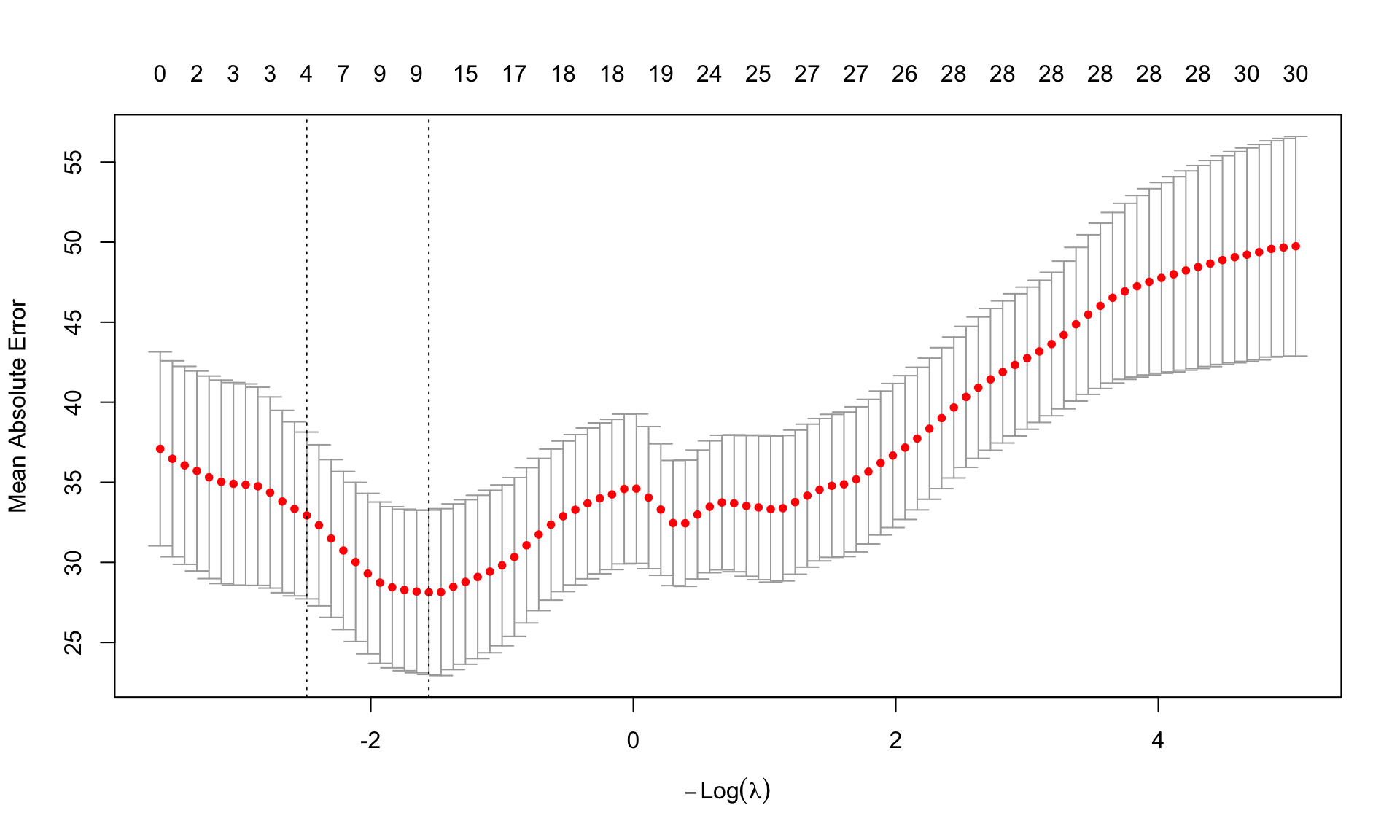
The horizontal axis of the plot shows different values of \(\lambda\) (by default, this is given in terms of \(log(\lambda)\) instead of \(\lambda\), which just makes the results easier to visualize). The vertical axis reports the associated cross-validation error. Across the top of the plot, we can also see the number of variables that are selected at each value of \(\lambda\). The dashed line on the left indicates the value of \(\lambda\) that achieves the minimum cross-validation error, which is what we would usually choose as our “final” model.
To print the values of \(\lambda\) corresponding to the minimum cross-validation error, we write
##
## Call:  cv.glmnet(x = x, y = y, type.measure = "mae")
##
## Measure: Mean Absolute Error
##
##     Lambda Index Measure    SE Nonzero
## min  4.749    23   28.13 5.133      10
## 1se 12.040    13   32.93 5.209       4
The table above shows that the cross-validation error is minimized at a value of \(\lambda = 4.7\), which produces a mean absolute error of $28 and selects 10 variables. A general rule of thumb is to select the value of \(\lambda\) that minimizes the error, but ultimately, the decision of which value of \(\lambda\) to use for the final model depends on your preference for how to balance model complexity and prediction error.
Forward selection, backward elimination, and LASSO regression are three common approaches to variable selection. An advantage of forward selection and backward elimination is that they do not require choosing a value of \(\lambda\) through cross-validation, which LASSO does. An advantage of LASSO is that it can be computationally much faster than stepwise regression when there are a large number of variables to choose from.
Regardless of which approach we use, it is important to remember there is no “one-size-fits-all” approach to variable selection. These methods should be used as helpful guides only, and we should always aim to incorporate background knowledge and domain expertise into the variable selection process wherever possible.