D Solutions

This Appendix contains some answers to end-of-chapter questions.

D.1 Answers for Chap. 1

Answer to Exercise 1.1.

1. Venn diagram?
2. $0.66$.
3. $0.13$.
4. $0.89$.
5. $0.4583...$
6. Not independent… but close.

Answer to Exercise 1.2.

1. $0.0587...$.
2. $0.3826...$.
3. $0.1887...$.
4. $1600/3201$.

Answer to Exercise 1.3.

1. $X \in \{(a, b, c) | (a, b, c) \in \mathbb{R}, a \ne 0\}$ where $\mathbb{R}$ represents the real numbers.
2. $R = \{ (a,b,c) \mid (a, b, c)\in \mathbb{R}, a\ne 0, b^2 - 4ac = 0\}$.
3. $Z = \{ (a,b,c) \mid (a, b, c)\in \mathbb{R}, a\ne 0, b^2 - 4ac < 0\}$.

Answer to Exercise 1.5.

1. $210$.
2. $165$.

Answer to Exercise 1.6.

Tree diagram: Fig, D.1; table: Table D.1; Venn diagram: Fig. D.2.

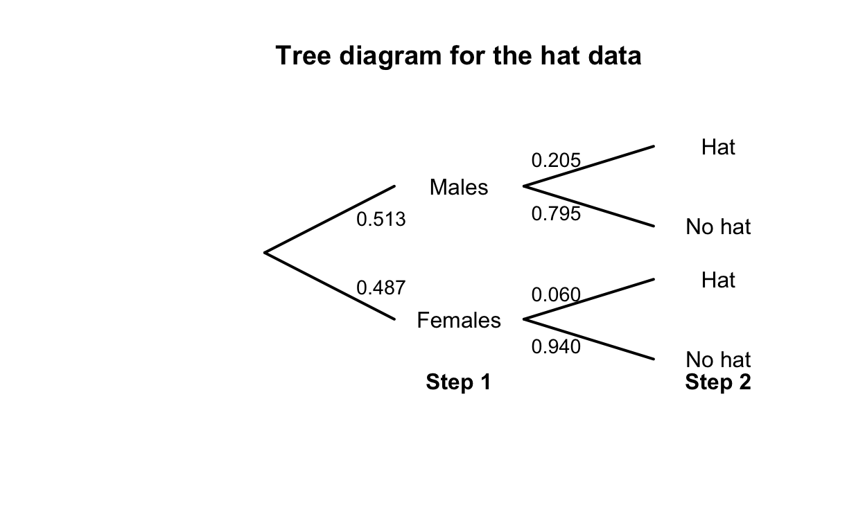
FIGURE D.1: Tree diagram for the hat-wearing example

TABLE D.1: The numbers of males and females wearing a hat in the middle of the day in Brisbane

	No Hat	Hat	Total
Males	307	79	386
Females	344	22	366

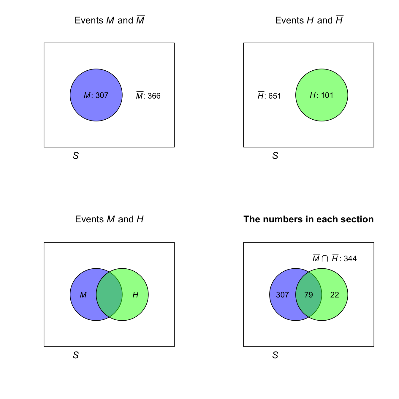
FIGURE D.2: The hat-wearing data as a Venn diagram

Answer to Exercise 1.7.

1. Choose one driver, and the other seven passengers can sit anywhere: $2!\times 7! = 10080$.
2. Choose one driver, and the other seven passengers can sit anywhere: $3!\times 7! = 30240$.
3. Choose one driver, choose who sits in what car sets, and the other five passengers can sit anywhere: $2!\times 2! \times 5! = 480$.

Answer to Exercise 1.11. Figure not shown.

Answer to Exercise 1.12.

1. $\Pr(\text{Player throwing first wins})$ means $\Pr(\text{First six on throw 1 or 3 or 5 or ...})$. So: $\Pr(\text{First six on throw 1}) + \Pr(\text{First six on throw 3}) + \cdots$. This produces a geometric progression that can be summed obtained (see App. A).
2. Use Theorem 1.6. Define the events $A = \text{Player 1 wins}$, $B_1 = \text{Player 1 throws first}$, and $B_2 = \text{Player 1 throws second}$.

Answer to Exercise 1.14.

Use Theorem 1.6 to find $\Pr(C)$ where $C = \text{select correct answer}$, $K = \text{student knows answer}$. Then, $\Pr(C) =\displaystyle {\frac{mp + q}{m}}$

Answer to Exercise 1.15. ???

Answer to Exercise 1.17.

1. Between $0$% and $8$%.
2. $0.20$.
3. $0.75$.

Answer to Exercise 1.18. The total number of children: $69\ 279$. Define $N$ as ‘a first-nations student’, $F$ as ‘a female student’, and $G$ as ‘attends a government school’.

1. $\approx 0.0870$.
2. $0.708$.
3. Approximately independent.
4. Approximately independent.
5. Not really independent.
6. Not really independent.
7. Not really independent.

Answer to Exercise 1.19.

1. The probability depends on what happens with the first card: $$\begin{align*} \Pr(\text{Ace second}) &= \Pr(\text{Ace, then Ace}) + |Pr(\text{Non-Ace, then Ace})\\ &= \left(\frac{4}{52}\times \frac{3}{51}\right) + \left(\frac{48}{52}\times \frac{4}{51}\right) \\ &= \frac{204}{52\times 51} \approx 0.07843. \end{align*}$$ You can use a tree diagram, for example.
2. Be careful:

$$\begin{align*} &\Pr(\text{1st card lower rank than second card})\\ &= \Pr(\text{2nd card a K}) \times \Pr(\text{1st card from Q to Ace}) + {}\\ &\qquad \Pr(\text{2nd card a Q}) \times \Pr(\text{1st card from J to Ace}) +{}\\ &\qquad \Pr(\text{2nd card a J}) \times \Pr(\text{1st card from 10 to Ace}) + \dots + {}\\ &\qquad \Pr(\text{2nd card a 2}) \times \Pr(\text{1st card an Ace}) \\ &= \frac{4}{51} \times \frac{12\times 4}{52} + {}\\ &\qquad \frac{4}{51} \times \frac{11\times 4}{52} +\\ &\qquad \frac{4}{51} \times \frac{10\times 4}{52} + \dots +\\ &\qquad \frac{4}{51} \times \frac{1\times 4}{52} \\ &= \frac{4}{51}\frac{4}{52}\left[ 12 + 11 + 10 + \cdots + 1\right]\\ &= \frac{4}{51}\frac{4}{52} \frac{13\times 12}{2} \approx 0.4705882. \end{align*}$$ 3. We can select any of the 52 cards to begin. Then, there are four cards higher and four lower, so a total of 16 options for the second card, a total of $52\times 16 = 832$ ways it can happen. The number of ways of getting two cards is $52\times 51 = 2652$, so the probability is $832/2652 \approx 0.3137$.

Answer to Exercise 1.20. No answer (yet).

Answer to Exercise 1.21. Write $x = Pr(A\cap B)$, so we have $x/0.4 + x/0.2 = 0.365$, giving $x = 0.05$.

Answer to Exercise 1.22. $k = 3$.

Answer to Exercise 1.22. $r = 2$.

Answer to Exercise 1.23.

1. Proceed:
   $$\begin{align*} \Pr(\text{at least two same birthday}) &= 1 - \Pr(\text{no two birthdays same}) \\ &= 1 - \Pr(\text{every birthday different}) \\ &= 1 - \left(\frac{365}{365}\right) \times \left(\frac{364}{365}\right) \times \left(\frac{363}{365}\right) \times \cdots \times \left(\frac{365 - n + 1}{365}\right)\\ &= 1 - \left(\frac{1}{365}\right)^{n} \times (365\times 364 \times\cdots (365 - n + 1) ) \end{align*}$$

2. Graph the relationship for various values of $N$ (from $2$ to $60$), using the above form to compute the probability.

3. How many people are needed to have at least a $50$% chance that at least two people share a birthday?

4. Birthdays are independent and randomly occur through the year (i.e., each day is equally likely).

N <- 2:80
probs <- array( dim = length(N) )

for (i in 1:length(N)){
  
  probs[i] <- 1 - prod( (365 - (1:N[i]) + 1)/365 )

}
plot( probs  ~ N,
      type = "l",
      lwd = 2,
      ylab = "Prob. at least two share birthday",
      xlab = expression(Group~size~italic(N)),
      las = 1)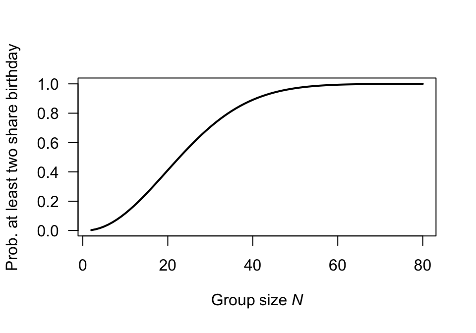

FIGURE D.3: Question 1

Answer to Exercise 1.31. $\approx 6.107$.

Answer to Exercise 1.32. $P = \{ (s, d) | s \in \{\text{<span class="larger-die">&#9857;</span>, <span class="larger-die">&#9859;</span>, <span class="larger-die">&#9861;</span>}\} \text{\ and\ } D \in \{ 2, 3, \dots, 10, \text{Jack}, \text{Queen}, \text{King}, \text{Ace}\} \}$.

Answer to Exercise 1.34. $\mathbb{R} \in \mathbb{C}$ but $\mathbb{C} \notin \mathbb{R}$

D.2 Answers for Chap. 2

Answer to Exercise 2.1.

1. $R_X = \{X \mid x \in (0, 1, 2) \}$; discrete.
2. $R_X = \{X \mid x \in (1, 2, 3\dots) \}$; discrete.
3. $R_X = \{X \mid x \in (0, \infty) \}$; continuous.
4. $R_X = \{X \mid x \in (0, \infty) \}$; continuous.
5. $R_X = \{X \mid x \in (0, 1, 2, \dots) \}$; discrete.
6. $R_X = \{X \mid x \in (0, 1, 2, \dots) \}$; discrete.
7. $R_X = \{X \mid x \in (0, \infty) \}$; continuous.

Answer to Exercise 2.2.

1. $\displaystyle F_X(x) = \begin{cases} 0 & \text{for $x < 10$};\\ 0.3 & \text{for $10 \le x < 15$};\\ 0.5 & \text{for $15 \le x < 20$};\\ 1 & \text{for $x \ge 20$}. \end{cases}$
2. $\Pr(X > 13) = 1 - F_X(13) = 0.7$.
3. $\Pr(X \le 10 \mid X\le 15) = \Pr(X \le 10) / \Pr(X \le 15) = F_X(10)/F_X(15) = 0.3/0.5 = 0.6$.

Answer to Exercise 2.3.

1. $\displaystyle F_Z(z) = \begin{cases} 0 & \text{for $z \le -1$};\\ 6z/15 - z^2/15 + 7/15 & \text{for $-1 < z < 2$};\\ 1 & \text{for $z \ge 2$}. \end{cases}$
2. $\approx 0.4666$.

:::{.answer} Answer to Exercise 2.4.

1. $\displaystyle p_W(w) = \begin{cases} 0.3 & \text{for $w = 10$};\\ 0.4 & \text{for $w = 20$};\\ 0.2 & \text{for $w = 30$};\\ 0.1 & \text{for $w = 40$};\\ 0 & \text{elsewhere}. \end{cases}$
2. $0.7$.

Answer to Exercise 2.5.

1. $\displaystyle f_Y(y) = \begin{cases} (4/3) - y^2 & \text{for $0 < y < 1$};\\ 0 & \text{elsewhere}. \end{cases}$
2. $0.625$.

Answer to Exercise 2.7.

Using the area of triangles, the ‘height’ is $2/27 \approx 0.07407407$ as shown below. Then, after some algebra: $$f_S(s) = \begin{cases} \frac{4}{81}s - \frac{14}{81} & \text{for $3.5 < s < 5$};\\ -\frac{4}{1377}s + \frac{122}{1377} & \text{for $5 < s < 30.5$}. \end{cases}$$ Also, $$F_S(s) = \begin{cases} 0 & \text{for $s < 3.5$};\\ \frac{(7 - 2s)^2}{162} & \text{for $3.5 < s < 5$};\\ \frac{2}{1377} (s^2 - 61s + 280) & \text{for $5 < s < 30.5$};\\ 1 & \text{for $s > 30.5$}. \end{cases}$$ Then, $\Pr(S > 20 \mid S > 10) = \Pr( (S > 20) \cap (S > 10) )/\Pr(S > 10) = \Pr(S > 20)/\Pr(S > 10) = 0.1601311 / 0.6103854$. This is about 0.2623.

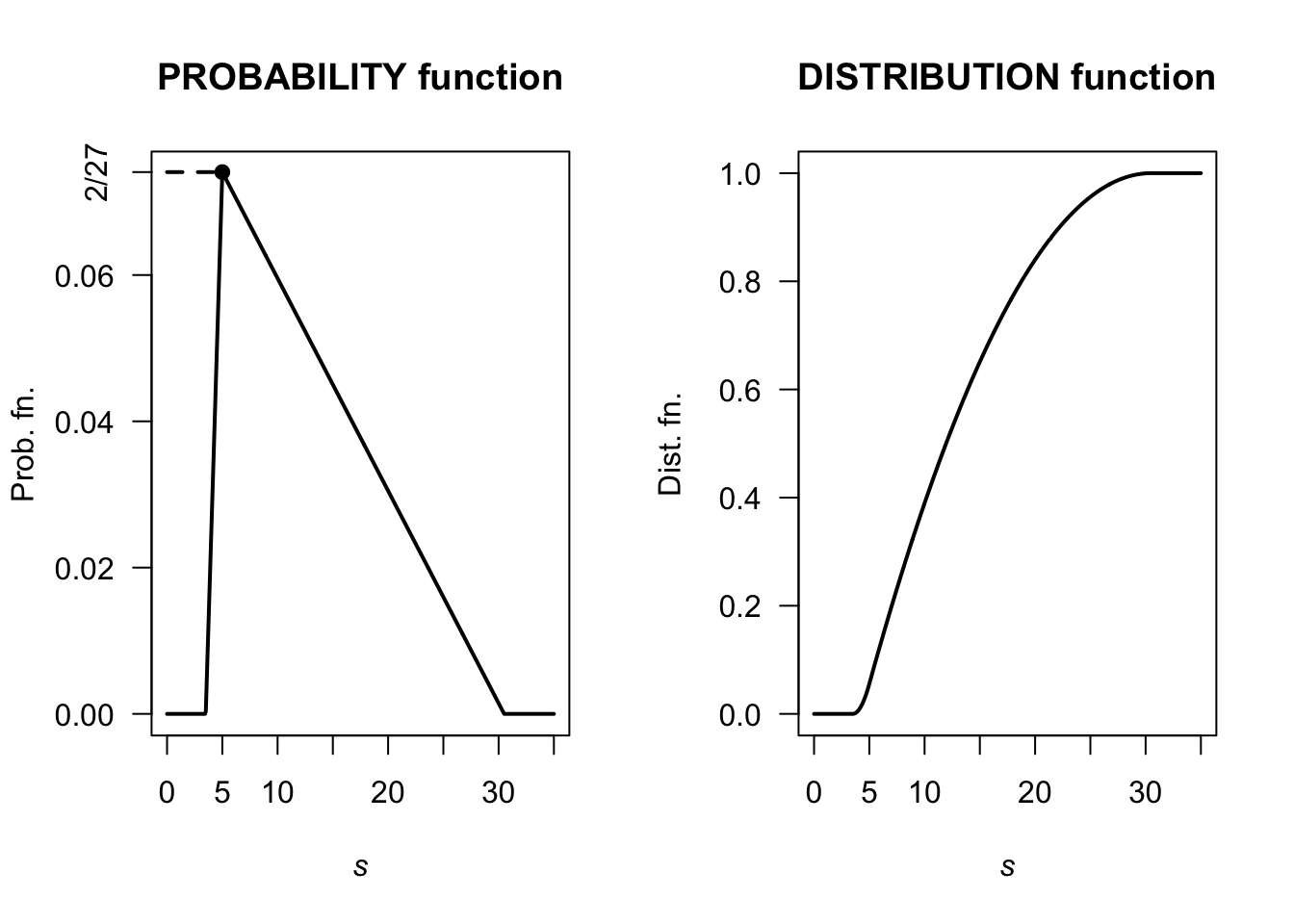
FIGURE D.4: A pdf and cdf

(1 - Fx(20) ) / ( 1 - Fx(10))
#> [1] 0.2623443

Answer to Exercise 2.8.

1. Producers usually need that they will receive at least a certain amount of rainfall.
2. A very poor graph below; I really have to fix that.
3. Six months have recorded over 60mm; so 6/81. But taking half of the previous ‘40 to under 60’ category, we’d get 12/81. So somewhere around there.
4. In June, there are 81 observations, so the median is the 41st: The median rainfall is between 0 to under 20mm.
   In December, there are 80 observations, so the median is the 40.5th: The median rainfall is between 40 to under 60mm.
5. Median; very skewed to the right.
6. …

#>       Buckets          Jun  Dec 
#>  [1,] "Zero"           "3"  "0" 
#>  [2,] "0 < R < 20"     "41" "17"
#>  [3,] "20 <= R < 40"   "19" "17"
#>  [4,] "40 <= R < 60"   "12" "21"
#>  [5,] "60 <= R < 80"   "2"  "9" 
#>  [6,] "80 <= R < 100"  "2"  "6" 
#>  [7,] "100 <= R < 120" "0"  "3" 
#>  [8,] "120 <= R < 140" "2"  "1" 
#>  [9,] "140 <= R < 160" "0"  "4" 
#> [10,] "160 <= R < 180" "0"  "0" 
#> [11,] "180 <= R < 200" "0"  "1" 
#> [12,] "200 <= R < 220" "0"  "1"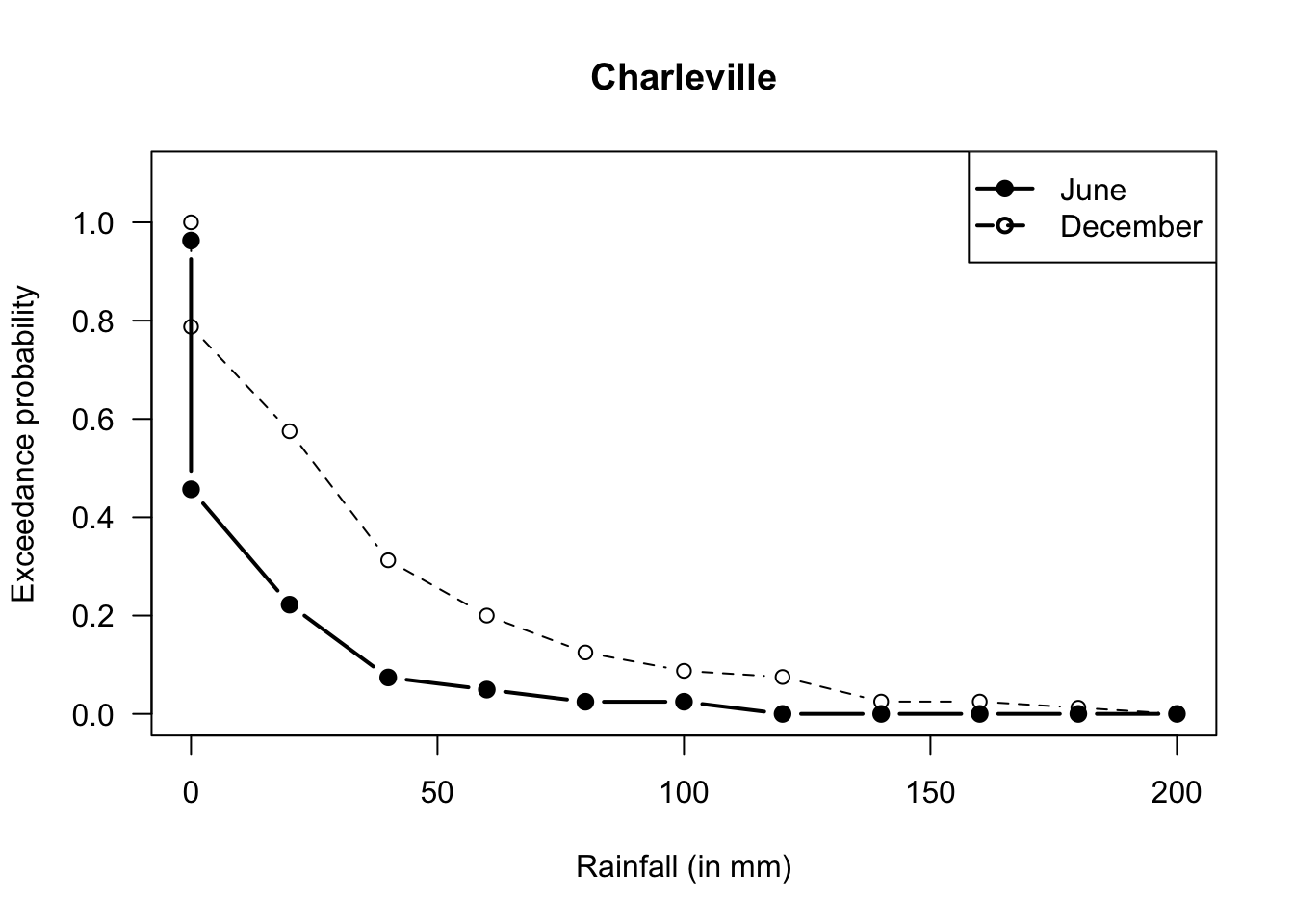

FIGURE D.5: Exceedance charts

Answer for Exercise 2.10.

1. $a\int_0^1 (1 - y)^2\,dy = \left. (1 - y)^3/3\right|_0^1 = 1/3$.
2. $\Pr(|Y - 1/2| > 1/4) = \Pr(Y > 3/4) + \Pr(Y < 1/4) = 1 - \Pr(1/4 < Y < 3/4) = 13/32$.
3. See Fig. D.6.

y <- seq(0, 1, length = 500)
fy <- ( (1 - y)^2 ) * 3

plot(fy ~ y,
     lwd = 2,
     xlab = "y",
     ylab = "PDF",
     type = "l")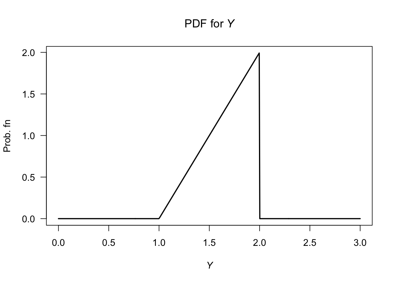

FIGURE D.6: The pdf of $y$

Answer for Exercise ??.

Exercise 2.11 df is:
$$F_Y()y) = \begin{cases} 0 & \text{for $y < 0$};\\ \frac{1}{3}(y - 1)^2 & \text{for $1 < y < 2$};\\ \frac{1}{3}(2y - 3) & \text{for $2 < y < 3$};\\ 1 & \text{for $y \ge 3$.} \end{cases}$$ When $y = 3$, expect $F_Y(y) = 1$; this is true. When $y = 1$, expect $F_Y(y) = 0$; this is true. For all $y$, $0 \le F_Y(y) \le 1$.

1. Write as $p(x) = \log_{10}(1 + x) - \log_{10}x$; then the sum is
   $$\begin{align*} (\log_{10}(2) - \log_{10} 1) + (\log_{10} 3 - \log_{10} 2) + (\log_{10} 4 - \log_{10} 3) + \dots\\ + (\log_{10} 9 - \log_{10} 8) + (\log_{10} 10 - \log_{10} 9) \end{align*}$$ and things cancel, leaving $\log_{10}10 = 1$.
2. DF:

Answer for Exercise 2.12. $\Pr(60 < Y < 70) = 154\,360\,000k/3\approx 51\,453\,333k$ and $\Pr(Y > 70) = 54\,360\,000k$. Using this model, the larger probability is dying over 70.

Answer to Exercise 2.15. $F_D(d) = \log (1 + d)$.

Answer for Exercise 2.17.

The pdf is $$f_X(x) = \frac{d}{dx} \exp(-1/x) = \frac{\exp(-1/x)}{x^2}$$ for $x > 0$. See Fig. D.7.

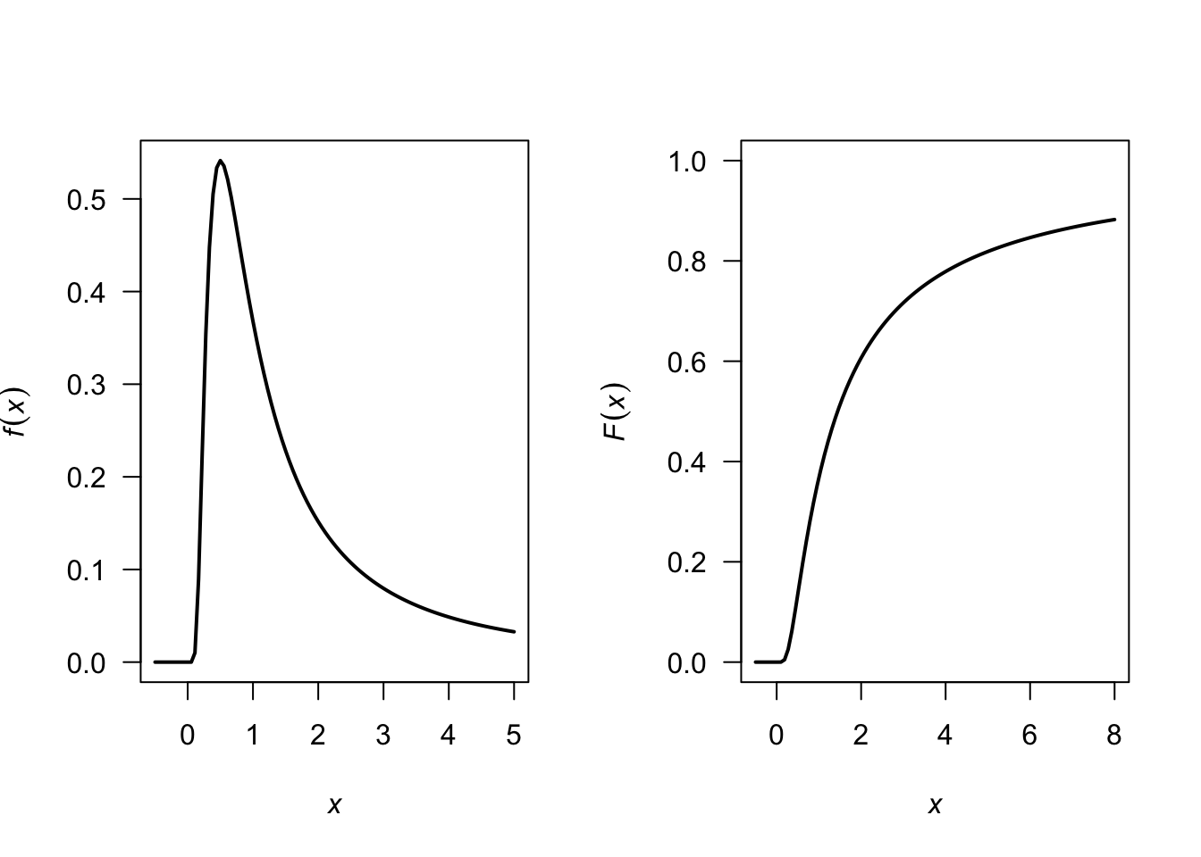
FIGURE D.7: A pdf

Answer for Exercise 2.18.

• 1 suit: Select 4 cards from the 13 of that suit, and there are four suits to select.
• 2 suits: There are two scenarios here:
  • Three from one suit, and one from another: Choose a suit, and select three cards from it: $\binom{4}{3}\binom{13}{3}$. Then we need another suit (three choices remain) and one card from (any of the 13).
  • Chose two suits, and two cards from each of two suits: $\binom{4}{2}\binom{13}{2}\binom{13}{2}$
• 3 suits: Umm…
• 4 suits: Choose one from each of the four suits.

One way to get 3 suits is to realise that the total probability must add to one…

### 1 SUIT
suits1 <- 4 * choose(13, 4) / choose(52, 4)

### 2 SUITS
suits2 <- choose(4, 3) * choose(13, 3) * choose(3, 1) * choose(13, 1) + 
          choose(4, 2) * choose(13, 2) * choose(13, 2)
suits2 <- suits2 / choose(52, 4)

### 4 SUITS:
suits4 <- choose(13, 1) * choose(13, 1) * choose(13, 1) * choose(13, 1)
suits4 <- suits4  / choose(52, 4)

suits3 <- 1 - suits1 - suits2 - suits4

round( c(suits1, suits2, suits3, suits4), 3)
#> [1] 0.011 0.300 0.584 0.105

Answer for Exercise 2.19.

1. $a = 1/3$.
2. We find: $$F_Y(y) = \begin{cases} 0. & \text{for $t < 0$};\\ 1/3 & \text{for $t = 0$};\\ (1 - t + 3t^2 - t^3)/3 & \text{for $0 < t < 2$};\\ 1 & \text{for $t \ge 2$}. \end{cases}$$

D.3 Answers for Chap. 3

Answer for Exercise 3.1.

1. $k = -2$.
2. Not shown.
3. $\text{E}(Y) = 5/3$.
4. $\text{var(Y)} = 1/18$.
5. $\Pr(X > 1.5) = 3/4$.

Answer to Exercise 3.2. 1. $\text{E}(D) = 7/4$; $\text{var}(D) = 11/16$. 1. $M_D(t) = \exp(t)/2 + \exp(2t)/4 + \exp(3t)/4$.

Answer to Exercise 3.4.

1. $\text{E}(Z) = 0.6$. $\text{var}(Z) = 0.42$ (be careful with the derivatives here!)
2. $\Pr(Z = 0) = 0.49$, $\Pr(Z = 1) = 0.42$, $\Pr(Z = 2) = 0.09$.

Answer to Exercise 3.5.

1. $M'_G(t) = \alpha\beta(1 - \beta t)^{-\alpha - 1}$ so $\text{E}(G) = \alpha\beta$. $M''_G(t) = \alpha\beta^2(\alpha + 1)(1 - \beta t)^{-\alpha - 2}$ so $\text{E}(G^2) = \alpha\beta^2(\alpha + 1)$ and $\text{var}(G) = \alpha\beta^2$.

Answer to Exercise 3.6.

1. $2\left[ \frac{1}{r + 1} - \frac{1}{r + 2}\right]$.
2. $\text{E}((X + 3)^2) = 67/6$.
3. $\text{var}(X) = 1/18$.

Answer to Exercise 3.7.

1. $\int_2^\infty y\frac{2}{y^2}\,dy = 2\log y\Big|_2^\infty$ does not converge.
2. If $\text{E}(Y)$ is not defined, then $\text{var}(Y)$ cannot be defined either.
3. Not shown.
4. $F_Y(y) = 1 - (2/y)$.
5. Median is 4.
6. IQR is $8 - 8/3 = 16/3$.
7. $3/4$.

Answer to Exercise 3.8.

1. See Fig. D.8 (left panel).
2. Evaluate $F_X(t) = \displaystyle \int_{-\infty}^t \frac{1}{\pi(1 + x^2)}\,dx = \frac{1}{\pi}\arctan(x) + \frac{1}{2}$. See Fig. D.8 (right panel).
3. $\displaystyle \text{E}(X) = \int_{-\infty}^t \frac{x}{\pi(1 + x^2)}\,dx = ...$, which is not defined.

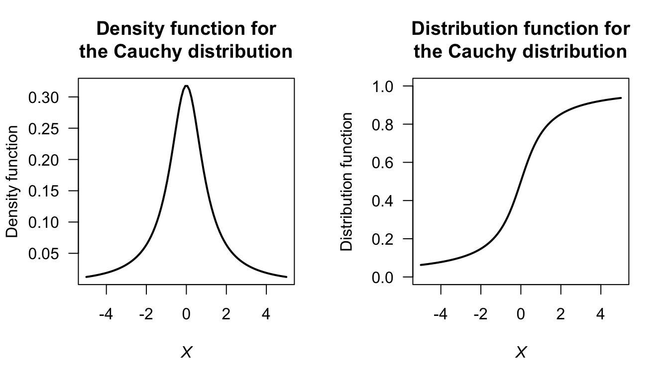
FIGURE D.8: The Cauchy distribution

Answer to Exercise 3.10.

Begin with Definition 3.13 for $M_X(t)$ and use fact that if a distribution is symmetric about 0 then $f_X(x) = f_X(-x)$ using symmetry. Transform the resulting integral.

Answer to Exercise 3.11.

First, the pdf needs to be defined (see Fig. D.9), and define $W$ as the waiting time. Let $H$ be the ‘height’ of the triangle. The area of triangle $A_1$ is $3H/4$, and the area of triangle $A_2$ is $51H/4$, so the value of $H$ is $2/27$.

The two lines, $L_1$ and $L_2$ can be found (find the slope; determine the linear equation) so that: $$f_W(w) = \begin{cases} 4w/81 - 14/81 & \text{for $3.5 < w < 5$};\\ -4w/1377 + 122/1377 & \text{for $5 \le w < 30.5$}. \end{cases}$$

1. $\text{E}(W)$ can be computed as usual across the two parts of the pdf: $\text{E}(W) = \frac{1}{4} + \frac{51}{4} = 13$ minutes.
2. $\text{E}(W^2)$ can be computed in two parts also: $\text{E}(W^2) = \frac{163}{144} + \frac{29\,699}{144} = 16598/8$. Hence $\text{var}(Y) = (1659/8) - 13^2 = 307/8\approx 38.375$, so the standard deviation is $\sqrt{38.375} = 6.19$ minutes.

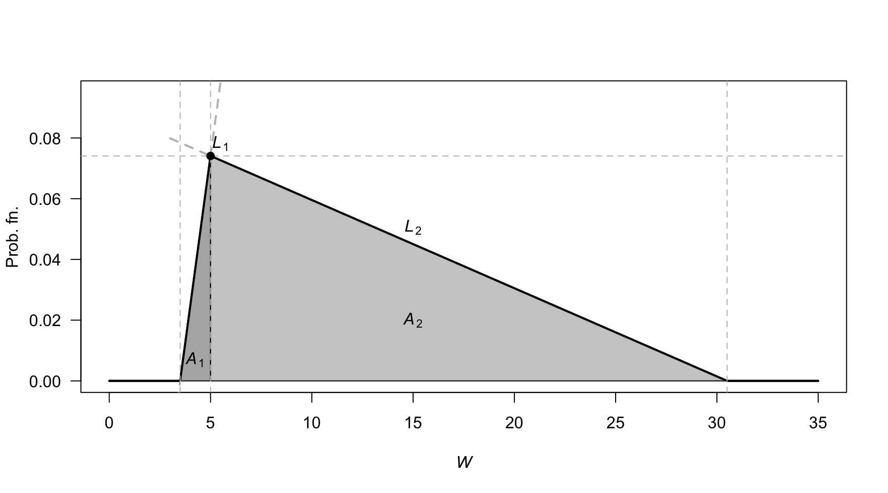
FIGURE D.9: Waiting times

Answer to Exercise 3.21.

1. $\text{E}(X) = \sum_{x = 1}^K x. p_X(x) = (1/6) + \sum_{x = 2}^K 1(x - 1)$. $\text{E}(X^2) = \frac{1}{K} + \sum_{x=2}^K \frac{x}{x - 1}$ with no closed form, so the variance is a PITA. No closed form!
2. See Fig. D.10.
3. Applying the definition:
   $$M_X(t) = \text{E}(\exp(tX)) = \frac{1}{K} + \left( \frac{\exp(2t)}{2\times 1} + \frac{\exp(3t)}{3\times 2} + \frac{\exp(4t)}{4\times 3} + \dots + \frac{\exp(Kt)}{K\times (K - 1)}\right).$$

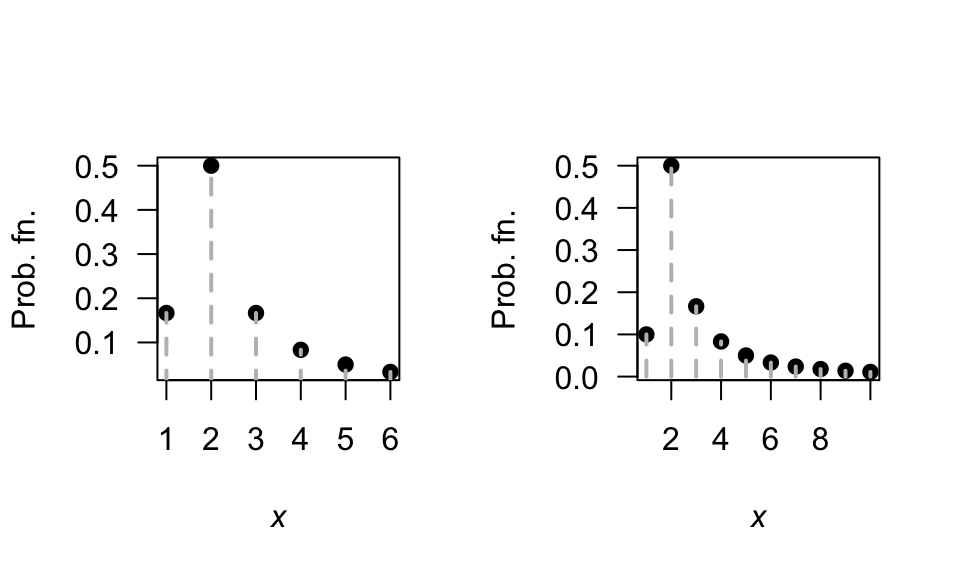
FIGURE D.10: The Soliton distribution

D.4 Answers for Chap. 4

Answer to Exercise 4.1. Show $\binom{n}{x} = \binom{n}{n - x}$ and hence $f_X(x)$ and $f_Y(y)$ are equivalent.

Answer to Exercise 4.2.

Care: The geometric is parameterised so that $x$ is the number of failures before a success (not the number of trails). Similarly for the negative binomial.

sum( dbinom(10:25, # Part 1
            size = 25,
            prob = 0.30) )
#> [1] 0.189436

sum( dbinom(0:9,  # Part 2
            size = 25,
            prob = 0.30) )
#> [1] 0.810564

sum( dbinom(5:10,  # Part 3
            size = 25,
            prob = 0.30) )
#> [1] 0.8117281

dgeom(x  = 5,  # Part 4: 5 fails before 1st success
      prob = 0.30)
#> [1] 0.050421

sum( dgeom(x  = 7:50,  # Part 5: Num. fails! 
           prob = 0.30) )
#> [1] 0.08235429

# Part 6; This means 5 fails, before 3rd success
dnbinom(x = 5,
        prob = 0.30,
        size = 3)
#> [1] 0.09529569

Answer to Exercise 4.4. 1. $0.0498$. 2. $0.0839$. 3. $0.446$.

Answer to Exercise 4.5.

4. $0.3401$.
5. $0.5232$.

Answer to Exercise 4.14.

Define $Y$ as the number of trials till the $r$th success, and hence $Y = X + r$.

1. $Y\in\{r, r + 1, r + 2, \dots\}$
2. $p_Y(y; p, r) = \binom{y - 1}{r - 1}(1 - p)^{y - r} p^{r - 1}$ for $y = r, r + 1, r + 2, \dots$.
3. $\text{E}(Y) = r/p$.
   $\text{var}(Y) = r(1 - p)/p^2$.
   

Answer to Exercise 4.16.

1. $0.25$.
2. dbinom(x = 2, size = 4, prob = 0.25) ${}= 0.2109375$.

Answer to Exercise 4.18. Suppose $X\sim\text{Pois}(\lambda)$; then $\Pr(X) = \Pr(X + 1)$ implies

$$\begin{align*} \frac{\exp(-\lambda)\lambda^x}{x!} &= \frac{\exp(-\lambda)\lambda^{x + 1}}{(x + 1)!} \\ \frac{\lambda^x}{x!} &= \frac{\lambda^{x} \lambda}{(x + 1) \times x!} \end{align*}$$ so that $\lambda = x + 1$ (i.e., $\lambda$ must be a while number). For example, if $x = 4$ we would have $\lambda = 5$. And we can check:

dpois(x = 4,     lambda = 5)
#> [1] 0.1754674

dpois(x = 4 + 1, lambda = 5)
#> [1] 0.1754674

Answer to Exercise 4.19.

1. $\text{E}(X) = kp$.
2. $\text{var}(X) = k p (1 - p) \times \left(\frac{N - k}{N - 1}\right)$.

Answer to Exercise 4.20.

Since $\text{var}(Y) = \text{E}(Y^2) - \text{E}(Y)^2$, find $\text{E}(Y^2)$ using (A.2):

$$\begin{align*} \text{E}(Y^2) &= \sum_{i = 0}^{b - a} i^2\frac{1}{b - a + 1}\\ &= \frac{1}{b - a + 1}(0^2 + 1^2 + 2^2 + \dots +(b - a)^2)\\ &= \frac{1}{b - a + 1}\frac{(b - a)(b - a + 1)(2(b - a) + 1)}{6}\\ &= \frac{(b - a)(2(b - a) + 1)}{6}. \end{align*}$$ Therefore $$\begin{align*} \text{var}(X) = \text{var}(Y) &= \frac{(b - a)(2(b - a) + 1)}{6} - \left(\frac{b - a}2\right)^2\\ &= \frac{(b - a)(b - a + 2)}{12}. \end{align*}$$

D.5 Answers for Chap. 5

Answer to Exercise 5.1.

For example: From $\mu = m/(m + n)$, we get $n = m(1 - \mu)/\mu$ and $m + n = m/\mu$. Also, from the expression for the variance, substitiute $m + n = m/\mu$ and simplify to get

$$n = \frac{\sigma^2 m (m + \mu)}{\mu^3}$$ Equate this expression for $n$ with $n = m(1 - \mu)/\mu$ from earlier, and solve for $m$. We get that $m = \frac{\mu}{\sigma^2}\left( \mu(1 - \mu) - \sigma^2\right)$; $n = \frac{1 - \mu}{\sigma^2}\left( \mu(1 - \mu) - \sigma^2\right)$.

Answer to Exercise 5.2.

1. $\text{E}(X) 51$km.h^$-1$. $\text{var}(X) = 147$(km.h^$-1$)².
2. Not shown.
3. $2/7$.
4. $7/12$.

Answer to Exercise 5.3.

1. About $2.$4% of vehicles are excluded.
2. $Y$ has the distribution of $X \mid (X > 30 \cap X < 72)$ if $X \sim N(48, 8.8^2)$. The pdf is

$$f_Y(y) = \begin{cases} 0 & \text{for $y < 30$};\\ \displaystyle \frac{1}{8.8k \sqrt{2\pi}} \exp\left\{ -\frac{1}{2}\left( \frac{y - 48}{8.8}\right)^2 \right\} & \text{for $30\le y \le 72$};\\ 0 & \text{for $y > 72$}. \end{cases}$$ where $k \approx \Phi(-2.045455) + (1 - \Phi(2.727273)) = 0.02359804$.

# Proportion excluded:
pnorm(30, 48, 8.8) + # Slower than 30
   (1- pnorm(72, 48, 8.8)) # Faster than 72
#> [1] 0.02359804

Answer to Exercise 5.4.

1. Not shown.
2. $\text{E}(X) \approx 38.4$ and $\text{var}(X) \approx 54.54$.
3. $\approx 0.870$.

Answer to Exercise 5.5.

1. Not shown.
2. About $0.0228$.
3. About $2.17$ kg/m^$3$.
4. About $2.21$ kg/m^$3$.

Answer to Exercise 5.7.

$\text{CV} = \frac{\sqrt{a\beta^2}}{\alpha\beta} = 1/\sqrt{\alpha}$, which is constant.

Answer to Exercise 5.8.

For the given beta distribution, $\text{E}(V) = 0.287/(0.287 + 0.926) = 0.2366...$ and $\text{Var}(V) = 0.08161874$.

1. $\text{E}(S) = \text{E}(4.5 + 11V) = 4.5 + 11\text{E}(V) = 7.10$ minutes. $\text{var}(S) = 11^2\times\text{Var}(V) = 9.875$ minutes².
2. See Fig. D.11.

v <- seq(0, 1, length = 500)

PDFv <- dbeta(v, shape1 = 0.287, shape2 = 0.926)

plot( PDFv ~ v,
      type = "l",
      las = 1,
      xlim = c(0, 1),
      ylim = c(0, 5),
      xlab = expression(italic(V)),
      ylab = "PDF",
      main = "Distribution of V",
      lwd = 2)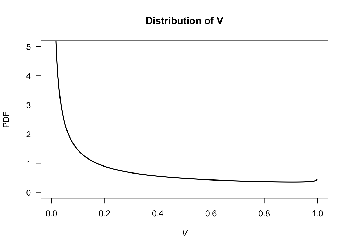

FIGURE D.11: Service times

Answer to Exercise 5.9.

1. $\text{E}[T] = 17.0$.
2. $\text{var}[T] = 16.5^2$.

Answer to Exercise 5.12.

4. In summer: If the event lasts more than 1 hour, what is the probability that it eventually lasts more than three hours?
5. In winter: If the event lasts more than 1 hour, what is the probability that it lasts less than two hours?

alpha <- 2; betaS <- 0.04; betaW <- 0.03
x <- seq(0, 1, length = 1000)

yS <- dgamma( x, shape = alpha, scale = betaS)
yW <- dgamma( x, shape = alpha, scale = betaW)

plot( range(c(yS, yW)) ~  range(x),
      type = "n", # No plot, just canvas
      las = 1,
      xlab = "Event duration (in ??)",
      ylab = "Prob. fn.")
lines(yS ~ x, 
      lty = 1,
      lwd = 2)
lines(yW ~ x, 
      lty = 2,
      lwd = 2)
legend( "topright",
        lwd = 2,
        lty = 1:2,
        legend = c("Summer", "Winter"))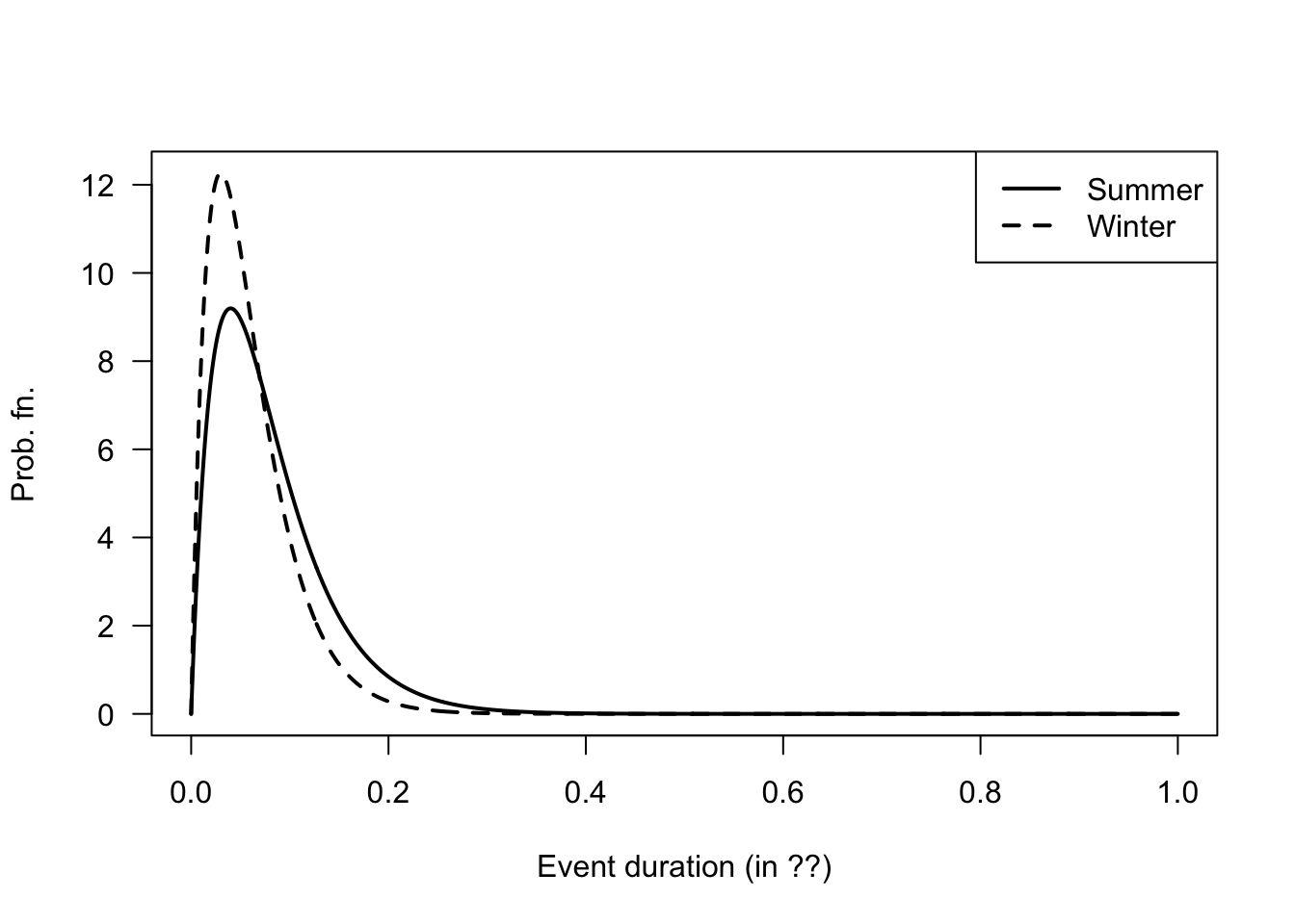

FIGURE D.12: Winter and summer

1 - pgamma(6/24, shape = alpha, scale = betaW)
#> [1] 0.002243448

1 - pgamma(6/24, shape = alpha, scale = betaS)
#> [1] 0.01399579

Answer to Exercise 5.23.

htMean <- function(x) {
  7.5 * x + 70
}
htSD <- function(x) {
  0.4575 * x + 1.515
}

NumSims <- 10000

Ages <- c(
  rep(2, NumSims * 0.32),
  rep(3, NumSims * 0.33),
  rep(4, NumSims * 0.25),
  rep(5, NumSims * 0.10)
)

Hts <- rnorm(NumSims,
             mean = htMean(Ages),
             sd = htSD(Ages))
hist(Hts,
     las = 1,
     xlab = "Heights (in cm)")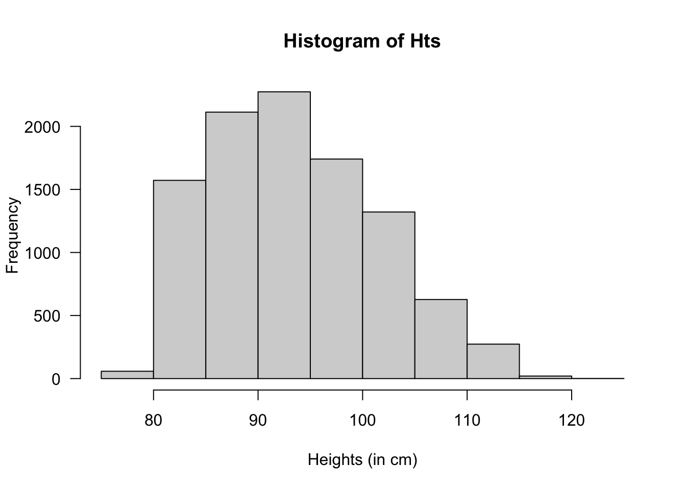

FIGURE D.13: Heights of children at day-care facilities

# Taller than 100:
cat("Taller than 100cm:", sum( Hts > 100) / NumSims * 100, "%\n")
#> Taller than 100cm: 22.42 %

# Mean and variance:
cat("Mean:", mean( Hts ), "cm; ",
    "Std dev: ", sd(Hts), "cm\n")
#> Mean: 93.52505 cm;  Std dev:  7.936301 cm

# Sort the heights to find where the tallest 20% are:
cat("Tallest 15% are taller than", 
    sort(Hts)[ NumSims * 0.85], "cm\n")
#> Tallest 15% are taller than 102.545 cm

D.6 Answers for Chap. 6

Answer to Exercise 6.1.

1. $5/24$.
2. $1/2$.
3. $1/4$.
4. Write: $$p_X(x) = \begin{cases} 7/24 & \text{if $x = 0$};\\ 17/24 & \text{if $x = 1$};\\ 0 & \text{otherwise}. \end{cases}$$
5. Only consider the column corresponding to $X = 1$: $$p_{Y\mid X = 1}(y\mid x = 1) = \begin{cases} (1/4)/(17/24) = 6/17 & \text{if $y = 0$};\\ (1/4)/(17/24) = 6/17 & \text{if $y = 1$};\\ (5/24)/(17/24) = 5/17 & \text{if $y = 2$};\\ 0 & \text{otherwise}. \end{cases}$$

Answer to Exercise 6.2.

1. $17$.
2. $7$.
3. $14$.
4. $38$.

Answer to Exercise 6.3.

1. $17$.
2. $7.2$.
3. $14$.
4. $36.8$.

Answer to Exercise 6.4. 1. $\text{E}(\overline{X}) = \text{E}([X_1 + X_2 + \cdots + X_n]/n) = [\text{E}(X_1) + \text{E}(X_2) + \cdots + \text{E}(+ X_n)]/n = [n \mu]/n = \mu$. 2. $\text{var}(\overline{X}) = \text{var}([X_1 + X_2 + \cdots + X_n]/n) = [\text{var}(X_1) + \text{var}(X_2) + \cdots + \text{var}(X_n)]/n^2 = [n \sigma^2]/n^2 = \sigma^2/n$.

Answer to Exercise ??.

1. Since $X + Y + Z = 500$, once the values of $X$ and $Y$ are known, the value of $Z$ has one specific value (i.e., all three values are not free to vary).
2. See Fig. D.14 (left panel).
3. See Fig. D.14 (right panel).
4. Proceed: $$\begin{align*} 1 &= \int_{200}^{300} \!\! \int_{100}^{400 - y} k\,dx\,dy + \int_{100}^{200} \!\! \int_{300 - y}^{400 - y} k\,dx\,dy \\ &= 30\ 000, \end{align*}$$ so that $k = 1/30\ 000$.

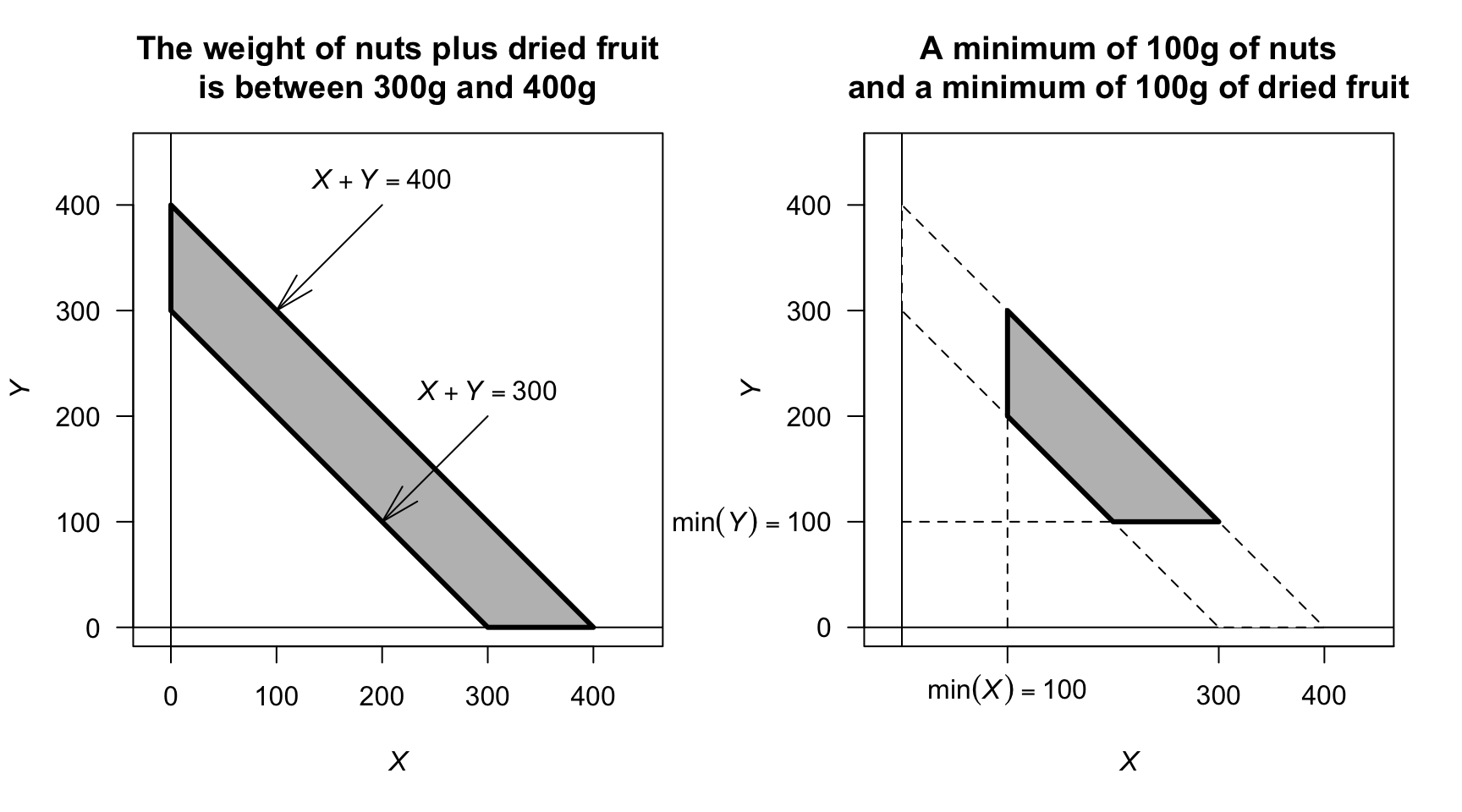
FIGURE D.14: The sample space for the mixture of nuts and dried fruit

Answer to Exercise 6.5.

For one month:

set.seed(932649)

NumRainEvents <- rpois(1,
                       lambda = 0.78)
MonthlyRain <- 0

if ( NumRainEvents > 0) {
     EventAmounts <- rgamma(NumRainEvents,
                           shape = 0.5,
                           scale = 6 )
     MonthlyRain <- sum( EventAmounts )
}

For 1000 simulations:

set.seed(932649)

MonthlyRain <- array(0,  
                     dim = 1000)

for (i in 1:1000){
 NumRainEvents <- rpois(1,
                       lambda = 0.78)
 MonthlyRain[i] <- 0

  if ( NumRainEvents > 0) {
       EventAmounts <- rgamma(NumRainEvents,
                             shape = 0.5,
                             scale = 6 )
       MonthlyRain[i] <- sum( EventAmounts )
  }
}

# Exact zeros:
sum(MonthlyRain == 0) / 1000
#> [1] 0.484

mean(MonthlyRain)
#> [1] 2.196798

mean(MonthlyRain[MonthlyRain > 0])
#> [1] 4.25736

Answer to Exercise 6.8.

1. Need integral to be one: $\displaystyle \int_0^1\!\!\!\int_0^1 kxy\, dx\, dy = 1$, so $k = 4$.
2. Here:
   $$4 \int_0^{3/8}\!\!\!\int_0^{5/8} kxy\, dx\, dy = 225/4096\approx 0.05493.$$

Answer to Exercise 6.9.

1. $\text{E}[U] = \mu_x - \mu_Z$; $\text{E}[V] = \mu_x - 2\mu_Y + \mu_Z$.
2. $\text{var}[U] = \sigma^2_x + \sigma^2_Z$; $\text{E}[V] = \sigma^2_x + 4\sigma^2_Y + \sigma^2_Z$.
3. Care is needed!
   $$\begin{align*} \text{Cov}[U, V] &= \text{E}[UV] - \text{E}[U]\text{E}[V]\\ &= \text{E}[X^2 - 2XY + XZ - XZ + 2YZ - Z^2] - \\ &\qquad (\mu_X^2 + 2\mu_X\mu_Y + \mu_X\mu_Z - \mu_X\mu_Z - 2\mu_Y\mu_Z - \mu^2_z)\\ &= (\text{E}[X^2] - \mu_X^2) - 2(\text{E}[XY] - \text{E}[X]\text{E}[Y]) + 2(\text{E}[YZ] - \mu_Y\mu_Z) -\\ &\qquad (\text{E}[Z^2] - \mu_Z^2)\\ &= \sigma^2_X - \sigma^2_Z, \end{align*}$$ since the two middle terms become $-2\text{Cov}[X, Y] + 2\text{Cov}[Y, Z]$, are both are zero (as given).
4. The covariance is zero if $\sigma^2_X = \sigma^2_Z$.

Answer to Exercise 6.10.

1. First find marginal distribution. Then $\text{E}(X | Y = 2) = 1/3$.
2. $\text{E}(Y \mid X\ge 1) = 12/5$.

Answer to Exercise 6.17.

1. Construct table (below) from listing all four outcomes.
2. We get $$p_X(x) = \begin{cases} 1/4 & \text{for $x = 0$};\\ 1/2 & \text{for $x = 1$};\\ 1/4 & \text{for $x = 2$}. \end{cases}$$
3. When given $Y = 1$, then the probability function is non-zero for $x = 1, 2$: $$p_{X|Y = 1}(x \mid Y = 1) = \begin{cases} 1/2 & \text{for $x = 1$};\\ 1/2 & \text{for $x = 2$}; \end{cases}$$
4. Not independent; for instance, when $Y = 0$, $\Pr(X) > 0$ for $x = 0, 1$, in constrast to when $Y = 1$.

.	$X = 0$	$X = 1$	$X = 2$
$Y = 0$	$1/4$	$1/4$	$0$
$Y = 1$	$0$	$1/4$	$1/4$

Answer to Exercise 6.19. Gamma distribution with parameters $n$ and $\beta$.

Answer to Exercise 6.21.

1. Adding: $$p_X(x) = \begin{cases} 0.40 & \text{for $x = 0$};\\ 0.45 & \text{for $x = 1$};\\ 0.15 & \text{for $x = 3$}. \end{cases}$$

2. $\Pr(X \ne Y) = 1 - \Pr(X = Y) = 1 - (0.20) = 0.80$.

3. $X < Y$ only includes these five $(x, y)$ elements of the sample space: $\{ (0, 1), (0, 2), (0, 3); (1, 2), (1, 3)\}$. The sum of these probabilities is 0.65.

   Then, given these five, only two of them sum to three (i.e., $(0, 3)$ and $(1, 2)$). So the probability of the intersection is $\Pr( \{0, 3\} ) + \Pr( \{1, 2\}) = 0.30$.

   So the conditional probability is $0.30/0.65 = 0.4615385$, or about 46%.

4. No: For $X = 0$, the values of $Y$ with non-zero probability are $Y = 1, 2, 3$. However, for $X = 1$ (for example), the values of $Y$ with non-zero probability are $Y = 1, 2$.

Answer to Exercise 6.26.

A table can be used to show the sample space (below). Looking for $X = 4$ we deduce that $$p_Y(y|X = 4) = \begin{cases} 2/7 = 0.2857 & \text{for $y = 1$};\\ 2/7 & \text{for $y = 2$};\\ 2/7 & \text{for $y = 3$};\\ 2/7 & \text{for $y = 4$};\\ 0 & \text{elsewhere}.\\ \end{cases}$$ Hence we deduce that $\text{E}[Y | X = 4] = 16/7\approx 2.2857$.

The table shows the values of $(x, y)$.

.	Die 1: 1	2	3	4	5	6
Die 2: 1	$(1, 1)$	$(2, 1)$	$(3, 1)$	$(4, 1)$	$(5, 1)$	$(6, 1)$
2	$(2, 1)$	$(2, 2)$	$(3, 2)$	$(4, 2)$	$(5, 2)$	$(6, 2)$
3	$(3, 1)$	$(3, 2)$	$(3, 3)$	$(4, 3)$	$(5, 3)$	$(6, 3)$
4	$(4, 1)$	$(4, 2)$	$(4, 3)$	$(4, 4)$	$(5, 4)$	$(6, 4)$
5	$(5, 1)$	$(5, 2)$	$(5, 3)$	$(5, 4)$	$(5, 5)$	$(6, 5)$
6	$(6, 1)$	$(6, 2)$	$(6, 3)$	$(6, 4)$	$(6, 5)$	$(6, 6)$

#> [1] 2.301363

Answer to Exercise 6.28.

annualRainfallList <- array( NA, dim = 1000)
for (i in 1:1000){
   rainAmounts <- array( 0, dim = 365) # Reset for each simulation

    wetDays <- rbinom(365, size = 1, prob = 0.32) # 1: Wet day
   locateWetDays <- which( wetDays == 1 )


   rainAmounts[locateWetDays] <- rgamma( n = length(locateWetDays),
                                         shape = 2,
                                         scale = 20)
   annualRainfallList[i] <- sum(rainAmounts)
}
# hist( annualRainfallList)

Days <- 1 : 365
prob <- (1 + cos( 2 * pi * Days/365) ) / 2.2

annualRainfallList2 <- array( NA, dim = 1000)
for (i in 1:1000){

  wetDays <- rbinom(365, size = 1, prob = prob) # 1: Wet day
  
  locateWetDays <- which( wetDays == 1 )
  
  rainAmounts2 <- array( 0, dim = 365)
  
  rainAmounts2[locateWetDays] <- rgamma( n = length(locateWetDays),
                                         shape = 2,
                                         scale = 20)
   annualRainfallList2[i] <- sum(rainAmounts2)
}
#hist( annualRainfallList2)

Days <- 1 : 365

probList <- array( dim = 365)
probList[1] <- 0.32

annualRainfallList3 <- array( NA, dim = 1000)

for (i in 1:1000){
  
  rainAmounts <- array( dim = 365 )

  for (day in 1:365) {
    if ( day == 1 ) {
      probList[1] <- 0.32
      wetDay <- rbinom(1, 
                       size = 1, 
                       prob = probList[1]) # 1: Wet day
      rainAmounts[1] <- rgamma( n = 1,
                                shape = 2,
                                scale = 20)

    } else {
    
      probList[i] <- ifelse( rainAmounts[day - 1] == 0,
                             0.15,
                             0.55)
      wetDay <- rbinom(1, 
                       size = 1, 
                       prob = probList[i]) # 1: Wet day

      if (wetDay) {
        rainAmounts[day] <- rgamma( n = 1,
                                    shape = 2,
                                    scale = 20)
      } else {
        rainAmounts[day] <- 0
      }
    }
  }
  annualRainfallList3[i] <- sum(rainAmounts)
    
}

#hist( annualRainfallList3)

Answer to Exercise 6.29.

1. Not shown.
2. Integrate correctly! $c = 1/2$.
3. $\Pr(X > 1) = 7/16 = 0.4375$. $P(Y < 1 \cap X > 1) = 7/16$. Then, $P(Y < 1 \mid X > 1) = 1$, which makes sense from the diagram (if $X > 1$, $Y$ must be less than 1).
4. $P(Y < 1 \mid X > 0.25) = P(Y < 1 \cap X > 0.25)/\Pr(X > 0.25)$.
5. $\frac{13}{16}\approx 0.8125$.

D.7 Answers for Chap. 7

Answer to Exercise 7.1.

For $0 < x < 2$, the transformation is one-to-one. The inverse transform is $X = Y^{1/3}$, and so $0 < y < 8$.

Pdf of $Y$ is $$f_Y(y) = \begin{cases} y^{-1/3}/6 & \text{for $0 < y < 8$};\\ 0 & \text{otherwise}. \end{cases}$$

:::{.answer} Answer to Exercise 7.2.

1. Table not shown.
2. Find: $$f_{Y_1}(y_1) = \begin{cases} 1/2 & \text{if $y_1 = 1$};\\ 1/2 & \text{if $y_1 = 2$};\\ 0 & \text{otherwise}. \end{cases}$$

Answer to Exercise 7.3.

$Y \sim\text{Gam}(\sum\alpha, \beta)$.

Answer to Exercise 7.10.

1. First see that $Y = \log X$. Then:
   $$\begin{align*} F_Y(y) &= \Pr(Y < y) \\ &= \Pr( \exp X < y)\\ &= \Pr( X < \log y)\\ &= \Phi\big((\log y - \mu)/\sigma\big) \end{align*}$$ by the definition of $\Phi(\cdot)$.
2. Proceed: $$\begin{align*} f_Y(y) &= \frac{d}{dy} \Phi\big((\log y - \mu)/\sigma\big) \\ &= \frac{1}{y} \Phi\big((\log y - \mu)/\sigma\big) \\ &= \frac{1}{y\sqrt{2\pi\sigma^2}} \exp\left[\left( -\frac{ (\log y - \mu)^2}{\sigma}\right)^2\right] \end{align*}$$ since the derivative of $\Phi(\cdot)$ (the df of a standard normal distribution) is $\phi(\cdot)$ (the pdf of a standard normal distribution).
3. See Fig. D.15.
4. See below: About 0.883.

par( mfrow = c(2, 2))

x <- seq(0, 8,
         length = 500)

plot( dlnorm(x, meanlog = log(1), sdlog = 1) ~ x,
      xlab = expression(italic(y)),
      ylab = "PDF",
      type = "l",
      main = expression(Log~normal*":"~mu==1~and~sigma==1),
      lwd = 2,
      las = 1)
plot( dlnorm(x, meanlog = log(3), sdlog = 1) ~ x,
      xlab = expression(italic(y)),
      ylab = "PDF",
      type = "l",
      main = expression(Log~normal*":"~mu==3~and~sigma==1),
      lwd = 2,
      las = 1)
plot( dlnorm(x, meanlog = log(1), sdlog = 2) ~ x,
      xlab = expression(italic(y)),
      ylab = "PDF",
      main = expression(Log~normal*":"~mu==1~and~sigma==2),
      type = "l",
      lwd = 2,
      las = 1)
plot( dlnorm(x, meanlog = log(3), sdlog = 2) ~ x,
      xlab = expression(italic(y)),
      ylab = "PDF",
      main = expression(Log~normal*":"~mu==3~and~sigma==2),
      type = "l",
      lwd = 2,
      las = 1)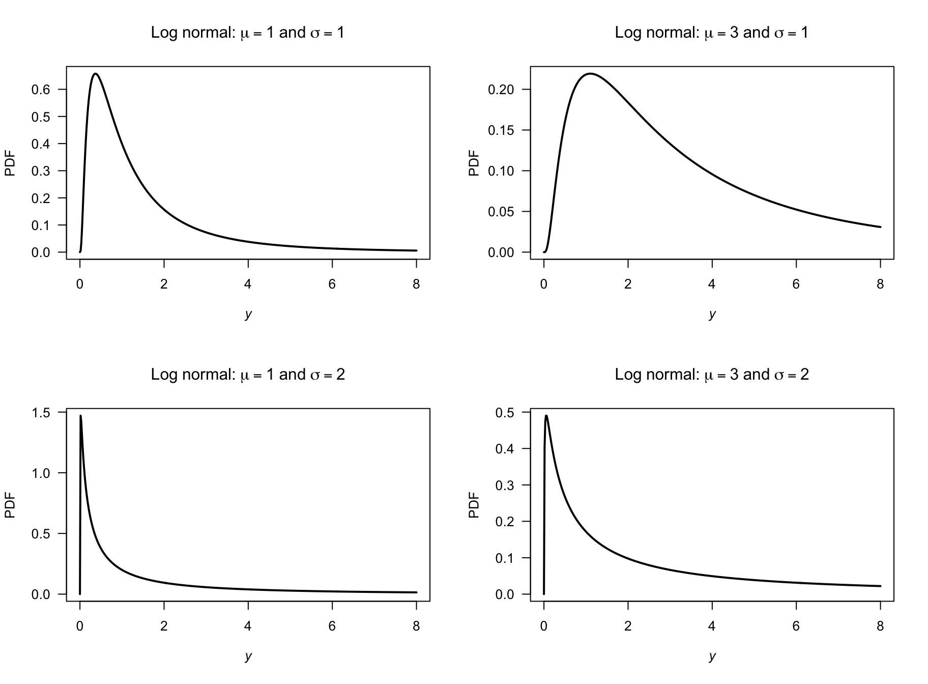

FIGURE D.15: Log-normal distributions

(1 - plnorm(2, meanlog=2, sdlog=2)) / 
  (1 - plnorm(1, meanlog=2, sdlog=2))
#> [1] 0.8834182

Answer to Exercise 7.11. $\Pr(Y = y) = \binom{4}{y^2} (0.2)^{y^2} (0.8)^{4 - y^2}$ for $y = 0, 1, \sqrt{2}, \sqrt{3}, 2$.

Answer to Exercise 7.16.

For the given beta distribution, $\text{E}(V) = 0.287/(0.287 + 0.926) = 0.2366...$ and $\text{Var}(V) = 0.08161874$.

1. $\text{E}(S) = \text{E}(4.5 + 11V) = 4.5 + 11\text{E}(V) = 7.10$ minutes. $\text{var}(S) = 11^2\times\text{Var}(V) = 9.875$ minutes².
2. $V\in (4.5, 15.5)$. See Fig. D.16.
3. This corresponds to $V = 10.5/11 = 0.9545455$, so $\Pr(S > 15) = \Pr(V > 0.9545455) = 0.01745087$.
4. With $V$, the largest 20% correspond to $V = 0.004080076$, so that $S = 4.544881$; the quickest 20% are within 4.54 minutes.

v <- seq(0, 1, length = 500)
stime <- 4.5 + 11 * v
  
PDFv <- dbeta(v, shape1 = 0.287, shape2 = 0.926)

plot( PDFv ~ stime,
      type = "l",
      las = 1,
      xlim = c(0, 15.5),
      ylim = c(0, 5),
      xlab = expression(italic(S)),
      ylab = "PDF",
      main = "Distribution of S",
      lwd = 2)
abline(v = 4.5,
       lty = 2,
       col = "grey",
       lwd = 2)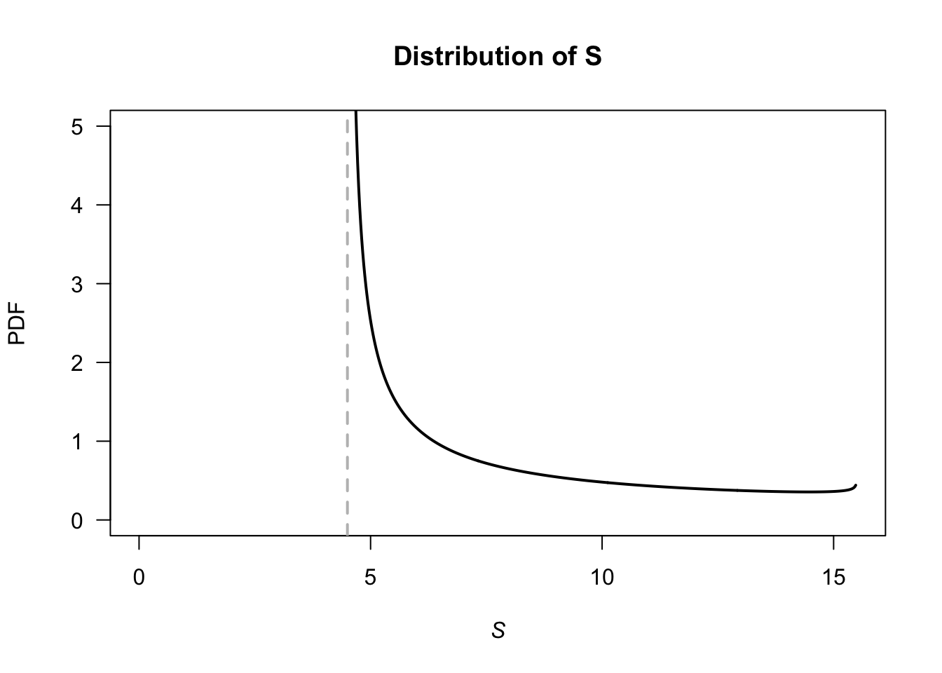

FIGURE D.16: Service times

## Part 3
1 - pbeta( 0.9545455, shape1 = 0.287, shape2 = 0.926)
#> [1] 0.01745087

## Part 4
qbeta(0.2, shape1 = 0.287, shape2 = 0.926) + 4.5
#> [1] 4.50408

D.8 Answers for Chap. 8

Answer to Exercise 8.3.

$\text{E}(Y) = \int_0^1 y(3y^2)\, dy = 3/4$. $\text{E}(Y^2) = 3/5$, so $\text{Var}(Y) = 3/80$. By the CLT, $\overline{Y}\sim N(3/4, 3/(80n) )$. Therefore
$$\Pr\left( 3/4 - \sqrt{3/80} < \overline{Y} < 3/4 + \sqrt{3/80} \right) = \Pr\left( 0.56 < \overline{Y} < 0.94 \right)$$ is needed. For a sample of size $n$,
$$\Pr\left( \frac{0.56 - 0.75}{0.19/\sqrt{n}} < Z < \frac{0.56 - 0.75}{0.19/\sqrt{n}} \right) = \Pr(-\sqrt{n} < Z < \sqrt{n} )$$ which approaches one as $n\to\infty$. For example, if $n = 10$, $\Pr(-\sqrt{10} < Z < \sqrt{10} ) = 0.9984$.

Answer to Exercise 8.4.

Let the weight be $E$, so $E\sim N(59, 0.7)$. By the CLT, the sample mean $\overline{E} \sim N(59, 0.7/20)$. So
$$\Pr(\overline{E} > 59.5) = \Pr(Z > \frac{59.5 - 59}{\sqrt{0.7/20}}) = \Pr(z > 2.67) \approx 0.003792562.$$ 1. We seek $\Pr(s^2 > 1)$. Since
$$\frac{(n - 1)s^2}{\sigma^2}\sim \chi^2_{n - 1}$$ where $n = 12$ and $\sigma^2 = 0.7$. So
$$\begin{align*} \Pr(s^2 > 1) &= \Pr\left( \frac{11 s^2}{0.7} > \frac{11\times 1}{0.7} \right)\\ &=\Pr( \chi^2_{11} > 15.714)\\ &\approx 0.152. \end{align*}$$

Answer to Exercise 8.5.

Let the number broken be $B$, so $B \sim \text{Pois}(0.2)$.

1. The sample mean number (with $n = 20$) broken has the distribution $\overline{B}\sim N(0.2, 0.2/20)$ approx. So
   $$\Pr(B\ge 1) = \Pr\left( Z > \frac{1 - 0.2}{\sqrt{0.2/20}} \right) = \Pr(Z > 8) = 0.$$
2. In contrast, in any single carton, the probability of more than one broken egg is
   $$\Pr(B > 1) = 1 - \Pr(B = 0) = 1 - 0.8187 = 0.181$$ using the Poisson distribution.

Answer to Exercise 8.6.

1. $\text{E}(M) = 3/4$.
2. $\text{var}(M) = 3/80$.
3. $\overline{M}\sim N(3/4, 1/240)$.
4. $0.8788$.

D.9 Answers for Chap. 9

Answer to Exercise 9.1.

1. $f(\theta| y)\propto f(y\mid\theta)\times f(\theta)$, where (given):
   $$f(y\mid \theta) = (1 - \theta)^y\theta \quad\text{and}\quad f(\theta) = \frac{\theta^{m - 1}(1 - \theta)^{n - 1}}{B(m, n)}.$$ Combining then:
   $$f(\theta| y)\propto \theta^{(m + 1) - 1} (1 - \theta)^{(n + y) - 1}.$$ which is a beta distribution with parameters $m + 1$ and $n + y$.
2. Prior: $\text{E}(\theta) = m / (m + n) = 1.2/(1.2 + 2) = 0.375$. So then, $\text{E}(Y) = (1 - p)/p = 1.667$.
3. Posterior: $\text{E}(\theta) = (m + 1)/(m + 1 + n + y) = 0.3056$; slightly reduced.

---

Peter K. Dunn, 2024: CC BY-NC-SA 4.0