8 Sampling distributions
On completion of this module, students should be able to:
- use appropriate techniques to determine the sampling distributions of \(t\), \(F\), and \(\chi^2\) distributions.
- explain how the above distributions are related to the normal distribution.
- apply the concepts of the Central Limit Theorem in appropriate circumstances.
- use the Central Limit Theorem to approximate binomial probabilities by normal probabilities in appropriate circumstances.
8.1 Introduction
This chapter introduces the application of distribution theory to the discipline of statistics. Recall: distribution theory is about describing random variables using probability, and statistics is about data collection and extracting information from data.
8.2 From theoretical distributions to practical observations
Until now, our results have concerned theoretical probability distributions (i.e., distribution theory) that describe ideal distributions of infinite populations. In practice, of course, we do not have infinite populations, and we observe finite (usually relatively small) samples from unknown distributions.
Example 8.1 Suppose our population of interest is only female residents currently living in a local nursing home. (Usually, populations are much broader than this.) While the heights \(X\) of such residents may be described theoretically as, for example, \(X\sim N(170, 3^2)\), the actual heights of each of the \(N = 86\) female residents is one value from this theoretical distribution, and then rounded (for convenience) to the nearest centimetre.
For example, we may find the heights are: \(160\) cm; \(173\) cm; \(169\) cm; \(\ldots\); \(171\) cm.
So while heights are (in theory) continuous, we observe discrete values. Using these values then, the expected value (or population mean) height can be found as \[ \text{E}[X] = \mu = \sum_{i = 1}^{86} p_X(x_i) \times x_i \] using the formula for a discrete random variable (using Def. 3.1). Since the population contains \(N = 86\) equally-important observations, the expected value is \[ \text{E}[X] = \mu = \sum_{i = 1}^{86} \frac{1}{86} \times x_i. \] Using this same idea more generally, the population mean can be computed as \[ \mu = \frac{1}{N} \sum_{i = 1}^N x_i. \] Similarly, the variance of the population can be found as (Def. 3.5): \[ \sigma^2 = \frac{1}{N} \sum_{i = 1}^N (x_i - \mu)^2. \]
8.2.1 Estimating the population mean
Having all values of a population available is almost never possible, and we instead study a sample of size \(n\) from some probably-unknown distribution: \(x_1, x_2, \ldots, x_n\). Given the formula for computing value of the population mean, a sensible approach for computing the value of the sample would seem to be using \[ \bar{X} = \frac{1}{n}(X_1 + X_2 + \cdots X_n) = \frac{1}{n}\sum_{i=1}^n X_i. \] In turns out that this is a ‘good’ estimate of \(\mu\), in the sense that is an unbiased estimate of \(\mu\).
Definition 8.1 (Unbiased estimator) For some parameter \(\theta\), the estimate \(\hat{\theta}\) is called an unbiased estimator of \(\theta\) if \[ \text{E}[\hat{\theta}] = \theta. \]
This means that an unbiased estimator produces estimates that, on average, have the correct (population) value that they are estimating. This seems a sensible property for a ‘good’ estimator. (There are other properties of ‘good’ estimators too, we but do not explore these here.) When we say that \(\bar{X}\) is an unbiased estimator of \(\mu\) then, we mean that \(\text{E}[\bar{X}] = \mu\),
Theorem 8.1 (An unbiased estimator for $\mu$) The sample mean \[ \bar{X} = \frac{1}{n} \sum_{i = 1}^n X_i \] is an unbiased estimator of the population mean \(\mu\).
Proof. Using the definition of an unbiased estimator: \[\begin{align*} \text{E}[\bar{X}] &= \text{E}\left[ \frac{1}{n}(X_1 + X_2 + \cdots X_n) \right]\\ &= \frac{1}{n} \text{E}[ X_1 + X_2 + \cdots X_n ]\\ &= \frac{1}{n} \left( \text{E}[ X_1 ] + \text{E}[X_2] + \cdots \text{E}[X_n] \right) \\ &= \frac{1}{n} (n\times \mu) = \mu. \end{align*}\] That is, the expected value of \(\bar{X}\) is equal to \(\mu\). The estimator \(\bar{X}\) is an unbiased of \(\mu\).
8.2.2 Estimating the population variance
Similarly, given the formula for the population variance, we might suggest the following estimate of the population variance.
Theorem 8.2 (An unbiased estimator for $\sigma^2$) The sample variance \[\begin{equation} S^2_n = \frac{1}{n} \sum_{i=1}^n (X_i - \mu)^2. \tag{8.1} \end{equation}\] is an unbiased estimator of the population variance \(\sigma^2\).
Proof. Again starting with the definition of an unbiased estimator: \[\begin{align*} \text{E}[S^2_n] &= \text{E}\left[ \frac{1}{n} \sum_{i=1}^n (X_i - \mu)^2\right]\\ &= \frac{1}{n} \text{E}\left[ (X_1 - \mu)^2 + (X_2 - \mu)^2 + \cdots + (X_n - \mu)^2\right]\\ &= \frac{1}{n} \left( \text{E}[ (X_1 - \mu)^2] + \text{E}[(X_2 - \mu)^2] + \cdots + \text{E}(X_n - \mu)^2\right]\\ &= \frac{1}{n} \left( \sigma^2 + \sigma^2 + \cdots + \sigma^2 \right)\\ &= \frac{1}{n} \times n\sigma^2 = \sigma^2. \end{align*}\] Thus, \(S^2_n\) is an unbiased estimator of \(\sigma^2\).
Equation (8.1) has a practical difficulty however; this equation is used to estimate the unknown value of the population variance, but relies on knowing the value of the population mean \(\mu\). Knowing the value of \(\mu\) but not the value of \(\sigma^2\) seems unlikely. Almost always, we would only have an estimate of the population mean \(\bar{X}\).
This may suggest using \[ \frac{1}{n} \sum_{i=1}^n (X_i - \bar{X})^2. \] to estimate the population variance. However, this estimate is not unbiased (ie., it is biased). Since \(\bar{X}\) estimates \(\mu\) imprecisely (from just one of the many possible samples), this introduces an extra source of variation into the estimation of \(\sigma^2\).
To see this, start again with the definition of an unbiased estimator: \[\begin{align*} \text{E}\left[ \frac{1}{n} \sum_{i=1}^n (X_i - \bar{X})^2 \right] &= \frac{1}{n}\text{E}\left[ \sum_{i=1}^n (X_i - \bar{X})^2\right]\\ &= \frac{1}{n}\text{E}\left[ \sum_{i=1}^n \left(X^2_i - 2X_i\bar{X} + \bar{X}^2\right)\right]\\ &= \frac{1}{n}\text{E}\left[ \sum_{i=1}^n X^2_i - \bar{X}\sum_{i=1}^n 2X_i + \sum_{i=1}^n \bar{X}^2\right]. \end{align*}\] Now observe that since \(\bar{X} = \sum_i X_i/n\), then \(\sum_i X_i = n \bar{X}\); hence \[\begin{align*} \text{E}\left[ \frac{1}{n} \sum_{i=1}^n (X_i - \bar{X})^2 \right] &= \frac{1}{n}\text{E}\left[ \sum_{i=1}^n X^2_i - \bar{X}^2 + n \bar{X}^2\right]\\ &= \frac{1}{n}\text{E}\left[ \sum_{i=1}^n X^2_i - n \bar{X}^2 \right]\\ &= \frac{1}{n}\left(\text{E}\left[ \sum_{i=1}^n X^2_i\right] - n\text{E}\left[ \bar{X}^2 \right]\right). \end{align*}\] This expression can be simplified by noting that \[ \text{var}[\bar{X}] = \text{E}[\bar{X}^2] - \text{E}(\bar{X})^2 = \text{E}[\bar{X}^2] - \mu^2, \] and so \(\text{E}[\bar{X}^2] = \text{var}{\bar{X}} + \mu^2 = \frac{\sigma^2}{n} + \mu^2\). Also, \[ \text{var}[X] = \text{E}[X^2] - \text{E}[X]^2 = \text{E}[X^2] - \mu^2, \] so that \(\text{E}[X^2] = \sigma + \mu^2\). Hence, \[\begin{align*} \text{E}\left[ \frac{1}{n} \sum_{i=1}^n (X_i - \bar{X})^2 \right] &= \frac{1}{n}\left(\text{E}\left[ \sum_{i=1}^n X^2_i\right] - n\text{E}\left[\sum_{i=1}^n \bar{X}^2 \right]\right)\\ &= \frac{1}{n}\left\{ \sum(\sigma^2 + \mu^2) - n\left(\frac{\sigma^2}{n} + \mu^2\right)\right\}\\ &= \frac{1}{n}\left\{ n\sigma^2 + n\mu^2 - \sigma^2 - n\mu^2\right\}\\ &= \frac{1}{n}\left\{ n\sigma^2 - \sigma^2\right\}\\ &= \frac{n - 1}{n} \sigma^2. \end{align*}\] Thus the estimator is a biased estimator of \(\sigma^2\). However, multiplying the estimator by \((n - 1)/n\) would produce an unbiased estimator.
Theorem 8.3 (An unbiased estimator for $\sigma^2$ ($\mu$ unknown)) When the value of \(\mu\) is unknown, an unbiased estimator of \(\sigma^2\) is \[\begin{equation} S^2_{n - 1} = \frac{1}{n - 1} \sum_{i=1}^n (X_i - \bar{X})^2. \tag{8.2} \end{equation}\] Notice that the divisor in front of the summation is now \(n - 1\) rather than \(n\).
Proof. Easily shown using the result above.
8.3 A example using a small population
8.3.1 Some results for samples
Suppose a simple random sample (SRS) of size \(n\) is taken from a population. The main interest is in the mean of the sample to estimate the unknown mean of the population \(\mu\). Typically, a population will be very large, and often it will not even be possible to list all elements of the population. However, for demonstration purposes, suppose the population contains only \(N = 5\) elements: \[ 2\qquad 3\qquad 3\qquad 4\qquad 8. \] From above, the mean of the population is \[ \mu = \frac{2 + 3 + 3 + 4 + 8}{5} = 4. \] Using R:
Similarly the variance of the population is \[ \sigma^2 = \frac{1}{N} \sum_{i = 1}^n (X_i - \mu)^2 = 4.4: \]
N <- length(Population)
sum( (Population - mean(Population))^2 ) / N
#> [1] 4.4

var(Population) * (N - 1) / N
#> [1] 4.4
The cumbersome second formula in R for the population variance is necessary because the R function var() computes the variance of a sample, rather than the variance of a population as we have here.
The factor \((n - 1)/n\) comes from the difference between the formulas (Sect. 8.2.2).
8.3.2 Distribution of the sample mean: \(n = 2\) (without replacement)
Assume we do not know the values of \(\mu\) and \(\sigma^2\), which is usually the case. Then, to estimate the value of \(\mu\), we take a sample of size \(n = 2\) from this population, without replacement. Because samples are taken at random, we do not know which elements will be in the sample, so we do not know what the value of \(\bar{X}\) will be.
Simple random sampling refers to all possible samples of size \(n\) being equally likely. Since there are \(\binom{N}{n}\) samples of size \(n\) when sampling without replacement from \(N\) objects, \(\binom{5}{2} = 10\) equally-likely possible samples of size \(n = 2\) are possible in this example. For instance, the sample \(\{2, 3\}\) has a probability of \(1/10\) of being selected, and the mean of this sample is \(2.5\).
We can use R to list all possible samples of size \(n = 2\) from the population:
### All possible combinations of 2 elements:
AllSamples <- combn(Population,
                    m = 2)
AllSamples
#>      [,1] [,2] [,3] [,4] [,5] [,6] [,7] [,8] [,9]
#> [1,]    2    2    2    2    3    3    3    3    3
#> [2,]    3    3    4    8    3    4    8    4    8
#>      [,10]
#> [1,]     4
#> [2,]     8

### Mean of each possible sample:
MeanAllSamples <- colMeans(AllSamples)
MeanAllSamples
#>  [1] 2.5 2.5 3.0 5.0 3.0 3.5 5.5 3.5 5.5 6.0
All \(10\) possible samples of size \(n = 2\) can be listed, with the mean of each sample:
cbind(                 t(AllSamples),
       "Sample mean" = MeanAllSamples,
       "Probability" = 1/10)
#>           Sample mean Probability
#>  [1,] 2 3         2.5         0.1
#>  [2,] 2 3         2.5         0.1
#>  [3,] 2 4         3.0         0.1
#>  [4,] 2 8         5.0         0.1
#>  [5,] 3 3         3.0         0.1
#>  [6,] 3 4         3.5         0.1
#>  [7,] 3 8         5.5         0.1
#>  [8,] 3 4         3.5         0.1
#>  [9,] 3 8         5.5         0.1
#> [10,] 4 8         6.0         0.1
The sample mean varies from sample to sample. The mean of a sample depends on which sample is selected at random.
From this information, the distribution of the sample mean itself can be determined (Fig. 8.1):
prop.table(table(MeanAllSamples))
#> MeanAllSamples
#> 2.5   3 3.5   5 5.5   6
#> 0.2 0.2 0.2 0.1 0.2 0.1

plot( prop.table(table(MeanAllSamples)),
      las = 1,
      xlab = "Sample mean",
      ylab = "Probability",
      main = "The distribution of sample means")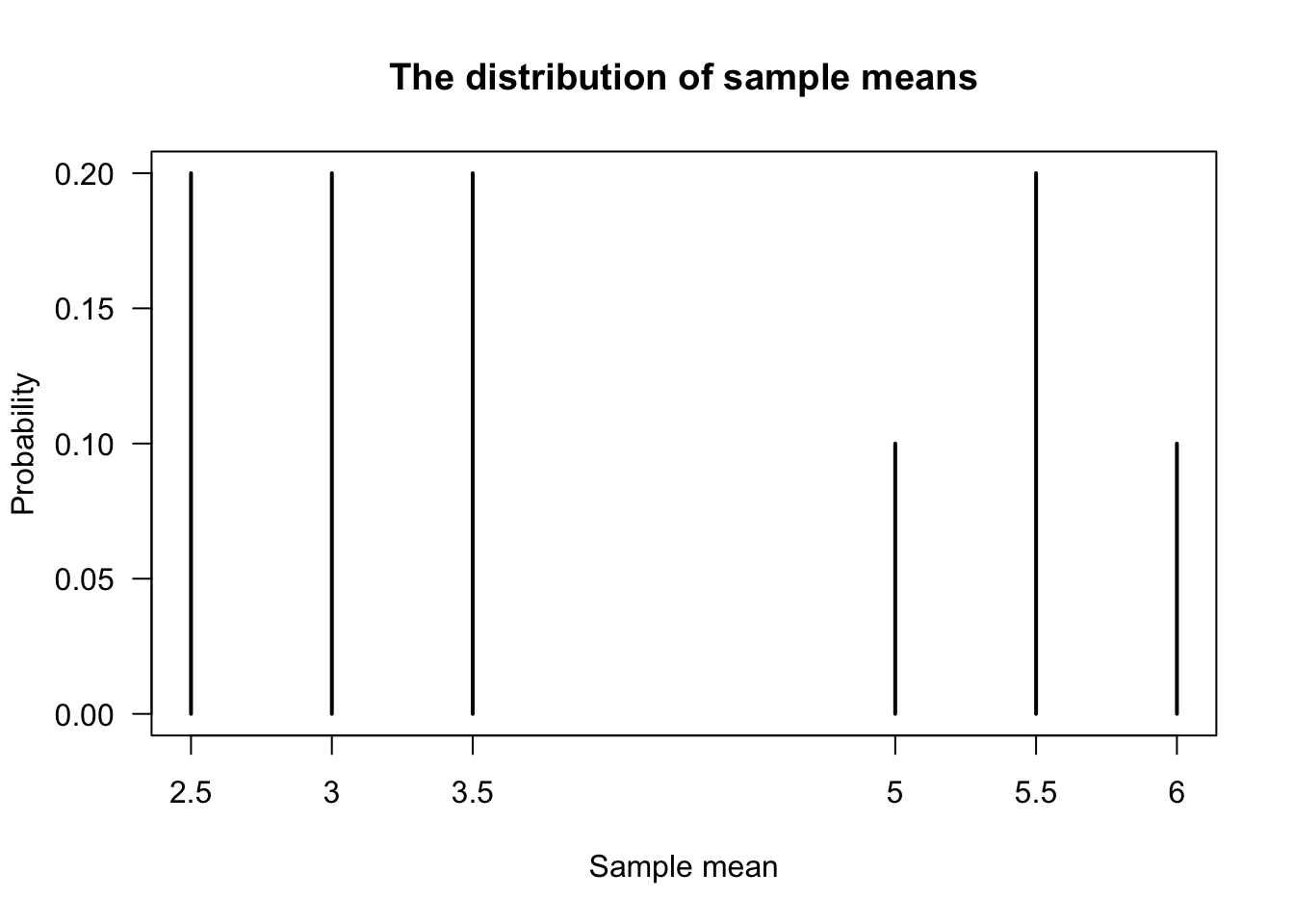
FIGURE 8.1: The distribution of the sample means
This distribution is known as the sampling distribution of the sample mean, recognising that the distribution is that of the sample mean.
The sample mean has a distribution: the value of the sample mean varies, depending on which sample is obtained.
The mean of the sampling distribution in Fig. 8.1 is \(\mu_{\bar{X}} = 4\):
mean(MeanAllSamples)
#> [1] 4
The variance of the sampling distribution in Fig. 8.1 is \(\sigma^2_{\bar{X}} = 1.65\):
Note that since we have the mean of all possible samples, we have the ‘population’ of sample means.
8.3.3 Distribution of the sample mean: larger samples (without replacement)
We can increase the sample size to \(n = 3\), and repeat:
### All possible combinations of 3 elements:
AllSamples <- combn(Population,
                    m = 3)

### Mean of each possible sample:
MeanAllSamples <- colMeans(AllSamples)
mean(MeanAllSamples)
#> [1] 4
n <- length(MeanAllSamples)
var(MeanAllSamples) * (n - 1) / n
#> [1] 0.7333333
The mean of all possible samples is the same (\(\mu_{\bar{X}} = 4\)), but the variance is smaller (\(\sigma^2_{\bar{X}} = 0.7333\) rather than \(1.65\)). For \(n = 4\), the mean of all possible samples remains the same, but the variance is smaller again:
8.3.4 Distribution of the sample mean: \(n = 2\) (with replacement)
All the above examples use sampling without replacement. However, sampling randomly with replacement could be used too. Then, there are \(5\times 5 = 25\) equally-likely samples possible:
AllSamplesWithReplacement <- expand.grid(Population, Population)
names(AllSamplesWithReplacement) <- c(NA,
                                      NA)
MeanAllSamplesWithReplacement <- rowMeans(AllSamplesWithReplacement)

cbind( AllSamplesWithReplacement[, 1],
       AllSamplesWithReplacement[, 2],
       "Sample mean" = MeanAllSamplesWithReplacement,
       "Probability" = 1/25)
#>           Sample mean Probability
#>  [1,] 2 2         2.0        0.04
#>  [2,] 3 2         2.5        0.04
#>  [3,] 3 2         2.5        0.04
#>  [4,] 4 2         3.0        0.04
#>  [5,] 8 2         5.0        0.04
#>  [6,] 2 3         2.5        0.04
#>  [7,] 3 3         3.0        0.04
#>  [8,] 3 3         3.0        0.04
#>  [9,] 4 3         3.5        0.04
#> [10,] 8 3         5.5        0.04
#> [11,] 2 3         2.5        0.04
#> [12,] 3 3         3.0        0.04
#> [13,] 3 3         3.0        0.04
#> [14,] 4 3         3.5        0.04
#> [15,] 8 3         5.5        0.04
#> [16,] 2 4         3.0        0.04
#> [17,] 3 4         3.5        0.04
#> [18,] 3 4         3.5        0.04
#> [19,] 4 4         4.0        0.04
#> [20,] 8 4         6.0        0.04
#> [21,] 2 8         5.0        0.04
#> [22,] 3 8         5.5        0.04
#> [23,] 3 8         5.5        0.04
#> [24,] 4 8         6.0        0.04
#> [25,] 8 8         8.0        0.04
From this table, the distribution of the sample mean itself can again be determined (Fig. 8.2):
prop.table(table(MeanAllSamplesWithReplacement))
#> MeanAllSamplesWithReplacement
#>    2  2.5    3  3.5    4    5  5.5    6    8
#> 0.04 0.16 0.24 0.16 0.04 0.08 0.16 0.08 0.04

plot( prop.table(table(MeanAllSamplesWithReplacement)),
      las = 1,
      xlab = "Sample mean",
      ylab = "Probability",
      main = "The distribution of sample means\n(sampling with replacement)")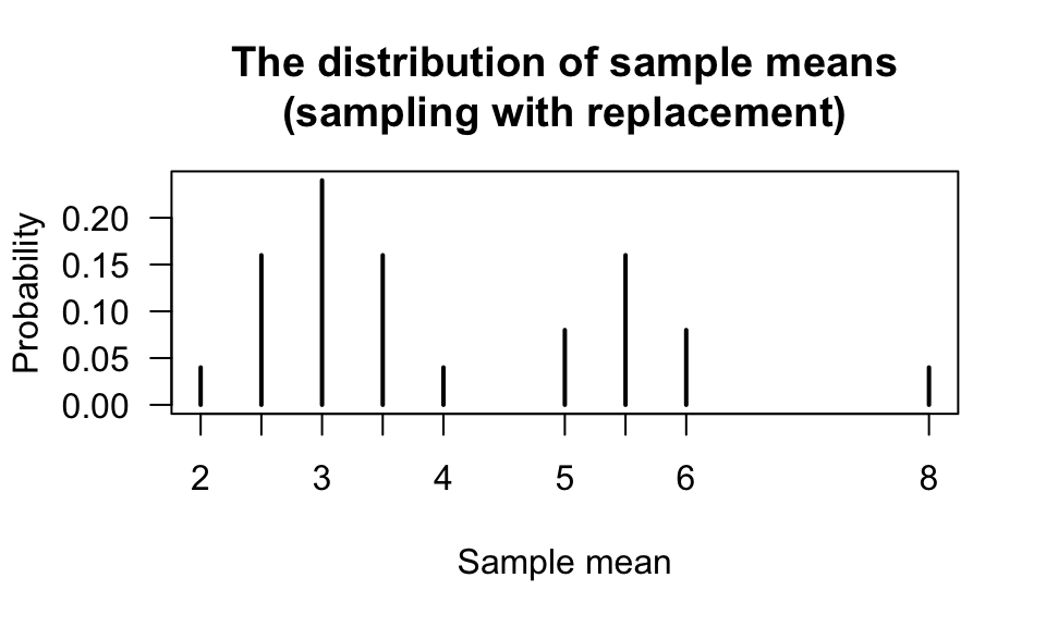
FIGURE 8.2: The distribution of the sample means
The mean and variance of the sampling distribution in this case are \(\mu_{\bar{X}} = 4\) and \(\sigma^2_{\bar{X}} = 2.2\) respectively:
8.3.5 The sampling distribution of other statistics
In principle, the distribution of any statistic could be found using the approach in the example above; that is, the median, variance, range, etc. all have a sampling distribution. For example, we can display the distribution of the sample range:
## Define a function to compute the range
myRange <- function(x){ max(x) - min(x) }

## The range of the population:
myRange(Population)
#> [1] 6

## Sampling:
AllSamplesWithReplacement <- expand.grid(Population, Population)
names(AllSamplesWithReplacement) <- c(NA,
                                      NA)
RangeAllSamplesWithReplacement <- apply(AllSamplesWithReplacement,
                                        1,
                                       "myRange")
prop.table(table(RangeAllSamplesWithReplacement))
#> RangeAllSamplesWithReplacement
#>    0    1    2    4    5    6
#> 0.28 0.32 0.08 0.08 0.16 0.08

plot( prop.table(table(RangeAllSamplesWithReplacement)),
      las = 1,
      xlab = "Sample range",
      ylab = "Probability",
      main = "The distribution of sample range\n(sampling with replacement)")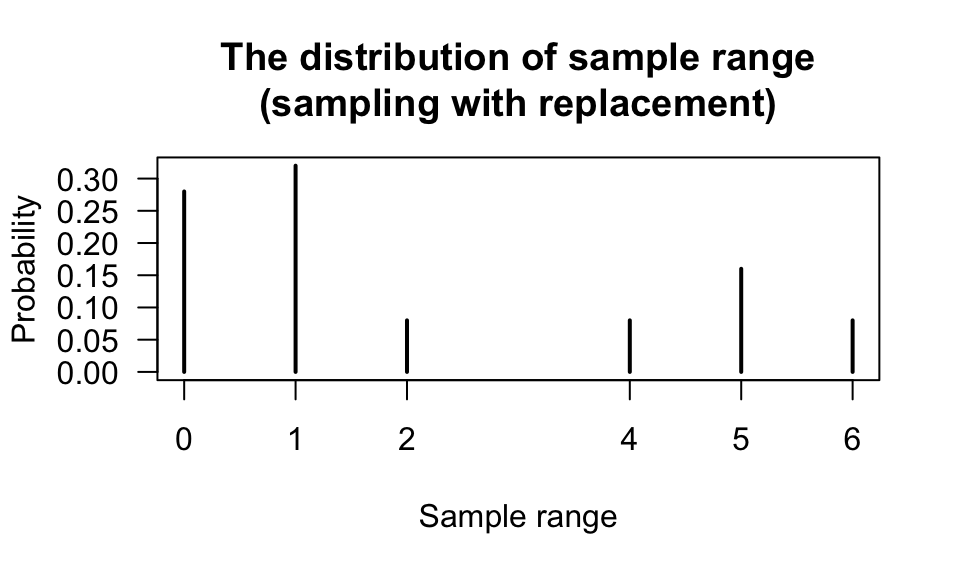
FIGURE 8.3: The distribution of the sample range
8.4 Sampling distributions
The previous section displays numerous sampling distributions: the distributions of sample statistics. In practice, populations are almost always very large and the number of possible samples huge, infinite, or the exact elements of the population difficult or impossible to list. In these cases, listing all possible samples and computing the exact sampling distributions is impossible.
In terms of distribution theory, the probability distributions in Figs. 8.1 and 8.2 are just the distribution of a random variable, since the sample mean is a random variable. Statistically, these distribution describe what to expect for the sample means when we randomly sample from a population.
Any quantity computed from a sample is a random variable, since its value is unknown beforehand. The observed value of the quantity depends on which sample is selected (at random).
Consequently, sample means, sample standard deviations, sample medians etc. all are random variables.
This knowledge is essential for extracting information from samples. Observe that the mean of the sampling distribution in the example (when taken without replacement) is the same as the mean of the population itself: \(\mu = (2 + 3 + 3 + 4 + 8 )/5 = 4\). Also, the variance of the sampling distribution is smaller than the variance of the population (\(\sigma^2 = 4.4\)). The exact relationship between \(\sigma^2_{\bar{X}}\) and \(\sigma^2\) is expanded on in Theorem 8.4.
Definition 8.2 (Statistic) A statistic is a real-valued function of the observations in a sample.
If \(X_1, X_2, \dots, X_n\) represents a numerical sample of size \(n\) from some population, then \(T = g(X_1, X_2, \dots, X_n)\) represents a statistic. Examples include the sample mean, sample standard deviation, sample variance and sample proportion. The individual observations in a sample are also statistics. Hence, for example, the minimum value in a sample (usually denoted \(\min\) or \(X_{[1]}\)), the maximum value, and the range \(\max - \min\) are statistics. Furthermore, even the first observation in a sample \(X_1\) is a statistic.
A random variable is a numeric variable which is fully determined by the values of all, some or even no members of the sample.
Example 8.2 (Sampling distribution of a statistic) The sampling distribution of a statistic is the theoretical probability distribution of the statistic associated with all possible samples of a particular size drawn from a particular population.
Notice that this definition is not confined to random samples. However, in practically all applications the sample involved is assumed to be random in some sense. Random sampling imposes a probability structure on the possible values of the statistic, allowing the sampling distribution to be defined.
We use \(\bar{X}\) to represent the mean of a sample whose value is as yet unknown (and depends on which sample is selected). The symbol \(\overline{x}\) is used to denoted the value of the sample mean, computed from the data found in a particular sample.
8.4.1 Random sampling
For our purposes, a random sample is defined as follows:
Definition 8.3 (Random sample) The set of random variables \(X_1, X_2,\dots,X_n\) is said to be a random sample of size \(n\) from a population with df \(F_X(x)\) if the \(X_i\) are identically and independently distributed (iid) with df \(F_X(x)\).
The definition uses the distribution function to accommodate both discrete and continuous random variables.
This definition of a random sample is standard in theoretical statistics. In statistical practice, however, many sampling designs are called “random”, such as simple random sampling, stratified sampling, and systematic sampling. These sampling methods produce ‘random samples’, even though the samples produced don’t necessarily satisfy Definition 8.3. Usually the context makes it clear whether the strict or loose meaning of ‘random sample’ is intended.
When a sample of size \(n\) is assumed to be chosen ‘at random’ without replacement from a population of size \(N\), this sample does not constitute a random sample in the sense of Definition 8.3. Even though each member of the sample has the same distribution as the population, the members of the sample are not independent. For example, consider the second element \(X_2\) of the samples in Sect. 8.1. Here, \(\Pr(X_2 = 2) = 0.2\) but that \(\Pr(X_2 = 2 \mid X_1 = 2) = 0\). Therefore \(\Pr(X_2 = 2 \mid X_1 = 2) \ne\Pr(X_2 = 2)\) and so \(X_2\) and \(X_1\) are dependent.
However, sampling at random without replacement approximates a random sample if the sample size \(n\) is small compared to the population size \(N\). In this case, the impact of removing some members of the population has minimal impact on the distribution of the population remaining, and the observations will be approximately independent. Populations sizes are commonly much larger than sample sizes (which we write as \(N>\!>n\)).
In Sect. 8.1, if the sampling is performed with replacement then \(\Pr(X_2 = 2 \mid X_1 = 2) = \Pr(X_2 = 2) = \Pr(X_1 = 2)\). Similar statements can be made for all sample members and all values of the population. In this case, the sample is a random sample according to Definition 8.3.
Sampling at random with replacement gives rise to a random sample, and sampling at random without replacement approximates a random sample provided \(N >\!> n\). Sampling without replacement when the sample size is not much smaller than the population size does not give rise to a random sample. This situation is often referred to as sampling from a finite population.
Sampling at random with replacement is also known as repeated sampling. A typical example is a sequence of independent trials (Bernoulli or otherwise) such as occur when a coin or die is tossed repeatedly. Each trial involves random sampling from a population, which in the case of a coin comprises H and T with equal probability.
Sampling from a continuous distribution is really a theoretical concept in which the population is assumed uncountably infinite. Consequently, sampling at random in this situation is assumed to produce a random sample.
8.4.2 The sampling distribution of the mean
Some powerful results exist to describe the sampling distribution of the mean of a random sample.
Theorem 8.4 (Sampling distribution of the mean) If \(X_1, X_2, \dots, X_n\) is a random sample of size \(n\) from a population with mean \(\mu\) and variance \(\sigma^2\), then the sample mean \(\bar{X}\) has a sampling distribution with mean \(\mu\) and variance \(\sigma^2 / n\).
Proof. This is a application of Corollary 6.1 with \(a_i = 1/n\).
Theorem 8.4 applies to a random sample as defined in Sect. 8.4.1. The remarkable feature of Theorem 8.4 is that the distribution of \(X\) is not important.
In Theorem 8.4, the distribution of the population from which the sample is drawn is irrelevant.
Theorem 8.4 applies to samples randomly selected with replacement from a finite population as described in Sect. 8.3.4. In the case where sample are taken without replacement, \(\mu_{\bar{X}}\) still equals \(\mu\) (as this result does not depend on the observations being independent), but \[\begin{equation} \text{var}(\bar{X}) = \frac{\sigma^2}{n} \times \frac{(N - n)}{(N - 1)} \end{equation}\] which is smaller than \(\sigma^2/n\) by the factor \((N - n)/(N - 1)\). This means that the standard deviation of \(\bar{X}\) is smaller than \(\sigma/\sqrt{n}\) by a factor of \(\sqrt{(N - n)/(N - 1)}\). (This factor was also seen in Exercise 4.19.)
Definition 8.4 (Finite Population Correction (FPC)) The finite population correction (FPC) factor is \[ \sqrt{ \frac{N - n}{N - 1} }. \]
Example 8.3 (Sampling without replacement) In Sect. 8.1, \(\mu = 4.4\) and \(\sigma^2 = 5.04\) for the population. The FPC is \[ \text{FPC} = \sqrt{ \frac{5 - 2}{5 - 1} } = 0.8660\dots. \] If sampling is done with replacement, then \(\mu_{\bar{X}} = \mu = 4.4\) and \(\text{var}(\bar{X}) = 2.52 = 5.04/2\), agreement with the theorem.
If sampling is done without replacement, the sampling distribution of the mean has mean \(\mu_{\bar{X}} = \mu = 4.4\) and variance \(\text{var}(\bar{X}) = 1.89 = \frac{5.04}{2} \times \text{FPC}^2\), in agreement with the note following Theorem 8.13.
Theorem 8.13 describes the location and spread of the sampling distribution of the mean, but not the shape of the sampling distribution. Remarkably, the shape of the sampling distribution only depends on the shape of the population distribution when the sample is small (Sect. 8.6).
8.5 Sampling distributions related to the normal distribution
8.5.1 General results
The normal distribution is used to model many naturally occurring phenomena (Sect. 5.3). Consequently, we begin by studying the sampling distributions of statistics of random samples that come from normal populations.
First, we present a useful result.
Theorem 8.5 (Linear combinations) Let \(X_1, X_2, \dots, X_n\) be a set of independent random variables where \(X_i\sim N(\mu_i,\sigma^2_i)\). Define the linear combination \(Y\) as \[ Y = a_1 X_1 + a_2 X_2 + \dots + a_nX_n. \] Then \(Y \sim N(\Sigma a_i\mu_i, \Sigma a^2_i\sigma^2_i)\).
Proof. In Theorem 5.2, the mgf of the random variable \(X_i\) was shown to be \[ M_{X_i} (t) = \exp\left\{\mu_i t + \frac{1}{2} \sigma^2_i t^2\right\}\quad\text{for $i = 1, 2, \dots, n$}. \] So, for a constant \(a_i\) (using Theorem 3.1 with \(\beta = 0\), \(\alpha = a_i\)): \[\begin{align*} M_{a_i X_i}(t) &= M_{X_i}(a_it)\\ &= \exp\left\{\mu_i a_i t + \frac{1}{2} \sigma^2_i a^2_i t^2\right\}. \end{align*}\] Since the mgf of a sum of independent random variables is equal to the product of their mgfs, then
\[\begin{align*} M_Y(t) &= \prod^n_{i = 1} \exp\left( \mu_i a_i t + \frac{1}{2} \sigma^2_i a^2_i t^2 \right)\\ &= \exp\left( t\Sigma a_i\mu_i +\frac{1}{2} t^2 \Sigma a^2_i \sigma^2_i \right). \end{align*}\] This is the mgf of a normal random variable with mean \(\text{E}(Y) = \Sigma a_i\mu_i\) and variance \(\text{var}(Y) = \Sigma a^2_i\sigma^2_i\).
Example 8.4 Theorem 8.5 can be demonstrated in R; see below.
set.seed(8979704) # For reproducibility
numberVars <- 1000 # That is: n

# The values of a_i, the coefficients in the linear combination
ai <- sample(x = seq(-2, 3),    # We select values of a_i between -2 and 3
             size = numberVars, # Need one for each X value
             replace = TRUE)    # Select with replacement

# The means of the individual distributions
mui <- runif(numberVars, # We take means from a uniform dist; one for each X
             min = -5,   # Min value is -5
             max = 5)    # Max value is 5
# The variances of the distributions
sigma2i <- runif(numberVars,  # Variance from a uniform distn also
                min = 1,    # Minimum values of 1
                max = 3)    # Maximum value of 3

# Compute the values directly:
Xi <- rnorm(numberVars,      # X_i with
            mean = mui,   # means
            sd = sqrt(sigma2i) )

# What we expect for Y = a_1 X_2 + a_2 X_2 + ...
# according to the Theorem:
Y <- ai * Xi  # The linear combination Y

# Show some:
someInfo <- cbind(ai, mui, sigma2i, Xi, Y)
someInfo[1:5, ]
#>      ai        mui  sigma2i        Xi         Y
#> [1,] -1  0.1690571 2.685062  1.993591 -1.993591
#> [2,]  1 -4.8907282 1.712808 -5.100795 -5.100795
#> [3,] -1 -0.4511475 1.562472 -1.184639  1.184639
#> [4,] -1  0.6878348 2.445416  4.870628 -4.870628
#> [5,] -2 -1.9851899 1.032315 -2.497384  4.994768


# Compare:
compareTable <- array( dim = c(2, 2) )
colnames(compareTable) <- c("Means:",
                            "Variances:")
rownames(compareTable) <- c("Using theorem",
                            "Computing directly")

compareTable[, 1] <- c( mean(ai * Xi),
                        mean(Y) )
compareTable[, 2] <- c( var(ai * Xi),
                        var(Y) )
compareTable
#>                        Means: Variances:
#> Using theorem      -0.2656963    32.6838
#> Computing directly -0.2656963    32.6838
The sampling distribution of the sum and mean of a random sample from a normal population follows directly from Theorem 8.5.
Corollary 8.1 (Sum and mean of a random sample) Let \(X_1, X_2, \dots, X_n\) be a random sample of size \(n\) from \(N(\mu,\sigma^2)\). Define the sum \(S\) and mean \(\bar{X}\) respectively as \[\begin{align*} S &= X_1 + X_2 + \dots + X_n\\ \bar{X} &= (X_1+X_2 + \dots + X_n)/n \end{align*}\] Then \(S\sim N(n\mu, n\sigma^2)\) and \(\bar{X}\sim N(\mu, \sigma^2/n)\).
Proof. Exercise.
Corollary 8.1 relies only on the population from which the sample is drawn having a normal distribution, and on the properties of expectation; it does not depend on the sample size \(n\). It is the basis for inference about the population mean of a normal distribution with known variance.
Example 8.5 (Sums of rvs) Suppose envelopes are collected into packs of \(25\) by weighing them. The weight of an envelope is distributed normally with mean 3 g and standard deviation \(0.6\) g. Any weighed pack of envelopes is declared as containing \(25\) if it weighs between \(70\) g and \(80\) g. What is the probability that a pile of \(25\) will not be counted as such?
Let random variable \(X_i\) be the weight of the \(i\)th envelope; then \(X_i \sim N(3, 0.36)\). Let \(Y = X_1 + X_2 + \dots + X_{25}\); then \(Y \sim N(75, 9)\). We require \(1 - \Pr(70 < Y < 80)\); see Fig. 8.4. Since the normal distribution is symmetric, proceed: \[\begin{align*} 1 - \Pr(70 < Y < 80) &= 2\times \Pr\left( Z < \frac{70 - 75}{\sqrt{9}} \right)\\ &= 2\times \Phi(-1.667) \\ &= 0.10. \end{align*}\] In R:
2 * ( pnorm( -1.667 ) )
#> [1] 0.0955144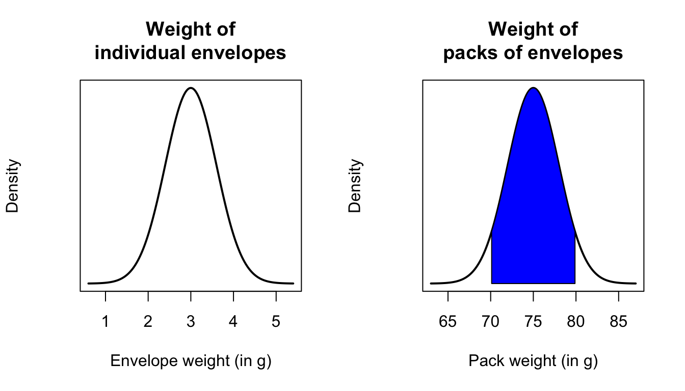
FIGURE 8.4: The envelope question. Left panel: The distribution of the weight of individual envelopes; right panel: The distribution of the weight of packs of \(25\) envelopes.
Example 8.6 (CLT) The IQs for a large population of \(10\) year-old boys (assumed normally distributed) were determined and found to have a mean of \(110\) and a variance of \(144\). How large a sample would have to be taken in order to have a probability of \(0.9\) that the mean IQ of the sample would not differ from the expected value \(110\) by more than \(5\)?
Let \(X_i\) be the IQ of the \(i\)th boy; then \(X_i \sim N(110, 144)\). Consider a sample of size \(n\) and let \(\bar{X} = \sum^n_{i = 1}X_i/n\); then \(\bar{X}\sim N(110, 144/n)\). Then \[ \Pr(|\bar{X} - 110|\leq 5) = 0.90. \] That is \[ \Pr\left(\frac{|\bar{X} - 110|\sqrt{n}}{12} \leq \frac{5\sqrt{n}}{12}\right) = 0.90 \] hence \[ \Pr(Z \leq 5\sqrt{n} /12) = 0.90. \] Using R:
z <- qnorm(0.95)
z
#> [1] 1.644854

n <- (z * 12 / 5) ^ 2
n
#> [1] 15.58393
The smallest size sample, then, would be a sample of \(n = 16\).
Example 8.7 (Two random variable) A certain product involves a plunger fitting into a cylindrical tube. The diameter of the plunger can be considered a normal random variable with mean \(2.1\) cm and standard deviation \(0.1\) cm. The inside diameter of the cylindrical tube is a normal random variable with mean \(2.3\) cm and standard deviation \(0.05\) cm. For a plunger and tube chosen randomly from a day’s production run, find the probability that the plunger will not fit into the cylinder.
Let \(X\) and \(Y\) be the diameter of the plunger and cylinder respectively. Then \(X\sim N\big(2.1, (0.1)^2\big)\) and \(Y\sim N\big( 2.3, (0.05)^2\big)\), and we seek \(\Pr(Y < X)\). The distribution of \(Y - X\) is \(N(2.3 - 2.1, 0.0025 + 0.01)\) so that, \[\begin{align*} \Pr(Y - X < 0) &= \Pr\left(Z <\frac{0 - 0.2}{\sqrt{0.0125}}\right) \quad\text{where $Z\sim N(0,1)$}\\ &= \Pr(Z < -1.78)\\ &= 0.0375. \end{align*}\] In R:
pnorm( -1.78 )
#> [1] 0.03753798
8.5.2 The \(\chi^2\) distribution
Having studied the sampling distribution of the mean, we now study the sampling distribution of the variance in a normal population. First, we present a useful result which is a variation of Theorem 7.4.
Theorem 8.6 (Chi-square distribution) Let \(X_1, X_2, \dots, X_n\) be a random sample of size \(n\) from \(N(\mu, \sigma^2)\). Then \(\sum_{i = 1}^n \left(\displaystyle{\frac{X_i - \mu}{\sigma}}\right)^2\) has a chi-square distribution with \(n\) degrees of freedom (df), written as \(\chi^2_n\).
Proof. If \(Z_i = \displaystyle{\frac{X_i - \mu}{\sigma}}\), then \[ \sum_{i = 1}^n \left(\frac{X_i - \mu}{\sigma}\right)^2 = \sum_{i = 1}^n Z_i^2. \] Here, \(Z_i\) is the standardised version of \(X_i\) and has a standard normal \(N(0, 1)\) distribution. Also, the random variables \(Z_i\) are independent because the \(X_i\) are independent (\(i = 1, 2, \dots, n\)). The required result follows directly from Theorem 7.4.
The four R functions for working with the \(\chi^2\) distribution have the form [dpqr]chisq(df), where df is the degrees of freedom (see Appendix B).
The sample variance is given by \[\begin{equation} S^2 = \frac{1}{n - 1}\sum_{i = 1}^n (X_i - \bar{X})^2. \tag{8.3} \end{equation}\] All sample estimates (‘statistics’) vary from sample to sample, so the sample variance has a distribution. The sampling distribution of the sample variance follows.
Theorem 8.7 (Distribution of the sample variance) Let \(X_1, X_2, \dots, X_n\) be a random sample of size \(n\) from \(N(\mu, \sigma^2)\). Then \[ \frac{(n - 1)S^2}{\sigma^2} \sim \chi^2_{n - 1}. \]
Proof. Only a partial proof is provided. Using (8.3), \[ \frac{(n - 1)S^2}{\sigma^2} = \sum_{i = 1}^n \left(\frac{X_i - \bar{X}}{\sigma}\right)^2, \] which looks much like the conditions for Theorem 8.6. The difference is that \(\bar{X}\) replaces \(\mu\). This difference is important: \(\mu\) is a fixed value that does not vary, whereas \(\bar{X}\) is a random variable that has a distribution.
Writing \[\begin{align*} \sum_{i = 1}^n \left( \frac{X_i - \bar{X}}{\sigma} \right)^2 &= \sum_{i = 1}^n \left( \frac{X_i - \bar{X} + \mu - \mu}{\sigma} \right)^2\\ &= \sum_{i = 1}^n \left( \frac{X_i - \mu}{\sigma} \right)^2 - n\frac{(\bar{X} - \mu)^2}{\sigma^2}. \end{align*}\] (Check!) Rewrite as \(V = W - U\) where \[ V = \sum_{i = 1}^n \left(\frac{X_i - \bar{X}}{\sigma}\right)^2;\qquad W = \sum_{i = 1}^n \left( \frac{X_i - \mu}{\sigma} \right)^2;\quad\text{and}\qquad U = n\frac{(\bar{X} - \mu)^2}{\sigma^2}.\qquad \] So we can write \(W = U + V\). Then observe:
- \(W \sim \chi^2_n\) by Theorem 8.6, so that the mgf of \(W\) is \(M_W(t) = (1 - 2t)^{-n}\).
- \(V \sim \chi^2_1\) because \(V\) is the square of a standard normal random variable, since \(\bar{X}\sim N(\mu, \sigma^2/n)\). Therefore, the mgf of \(V\) is \(M_V(t) = (1 - 2t)^{-1}\).
Provided \(W\) and \(V\) are independent, the mgf of \(W\) is the product of the mgfs of \(U\) and \(V\). This means that the mgf of \(U\) is \[ M_U(t) = \frac{M_W(t)}{M_V(t)} = (1 - 2t)^{n - 1} \] which is the mgf of the chi-square distribution with \(n - 1\) df.
This is only a partial proof, because the independence of \(U\) and \(V\) has not been shown.
Example 8.8 (Distribution of sample variance) A random sample of size \(n = 10\) is selected from the \(N(20, 5)\) distribution. What is the probability that the variance of this sample exceeds 10?
By Theorem 8.7, \[ \frac{(n - 1)S^2}{\sigma^2} = \frac{9 S^2}{5} \sim \chi^2_9. \] Therefore \[ \Pr(S^2 > 10) = \Pr\left( \frac{9S^2}{5} > \frac{9\times10}{5} \right) = \Pr(X^2 > 18), \] where \(X^2 \sim \chi^2(9)\). Using R, \(\Pr(S^2 > 10) = 0.03517\):
8.5.3 The \(t\) distribution
The basis of the independence assumed in the proof of Theorem 8.7 is the (perhaps surprising) result that the mean and variance of a random sample from a normal population are independent random variables.
Theorem 8.8 (Sample mean and variance: Independent) Let \(X_1, X_2,\dots, X_n\) be a random sample of size \(n\) from \(N(\mu, \sigma^2)\). Then the sample mean \[ \bar{X} = \frac1n\sum_{i=1}^n X_i \] and sample variance \[ S^2 = \frac{1}{n - 1}\sum_{i=1}^n (X_i - \bar{X})^2 \] are independent.
Proof. This proof is not given.
Another distribution that derives from sampling a normal population is the \(t\) distribution.
Definition 8.5 (T distribution) Suppose \(Z \sim N(0, 1)\) (i.e., a standard normal distribution) and \(V \sim \chi^2_n\) (i.e., a chi-squared distribution with \(n\) degrees of freedom). Then \[\begin{equation} T = \frac{Z}{\sqrt{V/n}} \tag{8.4} \end{equation}\] is defined as a \(T\) distribution with \(n\) degrees of freedom.
Definition 8.6 (T distribution) A continuous random variable \(X\) with probability density function \[\begin{equation} f_X(x) = \frac{\Gamma\left((\nu + 1)/2\right)}{\sqrt{\pi \nu}\,\Gamma(\nu/2)} \left(1 + \frac{x^2}{\nu}\right)^{-(\nu + 1)/2} \quad\text{for all $x$} \end{equation}\] is said to have a \(t\) distribution with parameter \(\nu > 0\). The parameter \(\nu\) is called the degrees of freedom. We write \(X \sim t_\nu\).
Proof. This proof is not given.
The pdf of the \(T\) distribution is very similar to the standard normal distribution (Fig. 8.5): bell-shaped and symmetric about zero. However, the variance is greater than one (Theorem 8.9) is dependent on \(\nu\).
The four R functions for working with the \(t\) distribution have the form [dpqr]t(df), where df is the degrees of freedom (see Appendix B).
FIGURE 8.5: Some \(t\) distributions (with normal distributions in dashed lines), with mean 0 and variance 1
Theorem 8.9 (Properties of the $T$ distribution) If \(X\sim t_\nu\) then
- For \(\nu > 1\), \(\text{E}(X) = 0\).
- For \(\nu > 2\), \(\text{var}(X) = \displaystyle{\frac{\nu}{\nu - 2}}\).
- The mgf does not exist because only the first \(\nu - 1\) moments exist.
Proof. This proof is not given.
Although we won’t prove it, as \(\nu\to\infty\) the \(t\) distribution converges to the standard normal (which can be seen in Fig. 8.5). In addition, from Theorem 8.9, we see that as \(\nu \to \infty\), \(\text{var}(X) \to 1\) as for the normal distribution.
The usefulness of the \(t\) distribution derives from the following result.
Theorem 8.10 ($T$-scores) Let \(X_1, X_2, \dots, X_n\) be a random sample of size \(n\) from \(N(\mu, \sigma^2)\). Then the random variable \[ T = \frac{\bar{X} - \mu}{S/\sqrt{n}} \] follows a \(t_{n - 1}\) distribution where \(\bar{X}\) is the sample variance and \(S^2\) is the sample variance as defined in (8.3).
Proof. We give a partial proof only. The statistic \(T\) can be written as \[\begin{align*} T &= \frac{\bar{X} - \mu}{S/\sqrt{n}}\\ &= \left(\frac{\bar{X} - \mu}{\sigma/\sqrt{n}}\right) \frac{1}{\sqrt{\frac{(n - 1)S^2}{\sigma^2}/(n - 1)}}\\ &= \frac{Z}{Y/(n - 1)}, \end{align*}\] where \(Z\) is a \(N(0, 1)\) variable and \(Y\) is a chi-square variable with \((n - 1)\) df. Using Definition 8.5 then, \(T\) has a \(T\) distribution.
Notice that \(T\) represents a standardised version of the sample mean. Because of this, the \(T\) statistic is important in statistical inference. You probably have used it is hypothesis testing, for example.
Example 8.9 (Calculating $T$) A random sample \(21, 18, 16, 24, 16\) is drawn from a normal population with mean of 20.
- What is the value of \(T\) for this sample?
- In random samples from this population, what is the probability that \(T\) is less than the value found above?
From the sample: \(\overline{x} = 19.0\) and \(s^2 = 12.0\). Therefore \(t = \frac{19.0 - 20}{\sqrt{12.0/5}} = -0.645\). (Notice lower-case symbols are used for specific values of statistics, and upper-case symbols for the random variables.)
Interest here is in \(\Pr(T < -0.645)\) where \(T\sim t_4\). From R, the answer is \(0.277\):
pt(-0.645, df = 4)
#> [1] 0.2770289
8.5.4 The \(F\) distribution
Definition 8.7 introduces the \(F\) distribution, which describes the ratio of two sample variances from normal populations. The \(F\) distribution is used in inferences comparing two sample variances. This distribution is also used in analysis of variance, a common technique used to test the equality of several means.
Definition 8.7 ($F$ distribution) A continuous random variable \(X\) with probability density function \[\begin{equation} f_X(x) = \frac{\Gamma\big( (\nu_1 + \nu_2)/2 \big) \nu_1^{\nu_1/2} \nu_2^{\nu_2/2} x^{(\nu_1/2) - 1}} {\Gamma(\nu_1/2)\Gamma(\nu_2/2)(\nu_1 x + \nu_2)^{(\nu_1 + \nu_2)/2}}\quad\text{for $x > 0$} \end{equation}\] is said to have an \(F\) distribution with parameters \(\nu_1 > 0\) and \(\nu_2 > 0\). The parameters are known respectively as the numerator and denominator degrees of freedom. We write \(X \sim F_{\nu_1, \nu_2}\).
Some \(F\) distributions are shown in Fig. 8.6. The basic properties of the \(F\) distribution are as follows.
Theorem 8.11 (Properties of $F$ distribution) If \(X\sim F(\nu_1, \nu_2)\) then
- For \(\nu_2 > 2\), \(\text{E}(F) = \displaystyle{\frac{\nu_2}{\nu_2-2}}\).
- For \(\nu_2 > 4\), \(\text{var}(F) = \displaystyle{\frac{2\nu_2^2(\nu_1 + \nu_2-2)} {\nu_1(\nu_2 - 2)^2(\nu_2 - 4)}}\).
- The mgf does not exist.
Proof. Not covered.
FIGURE 8.6: Some \(F\) distributions
The relationship between the \(T\) and \(F\) distribution can be established. Using Equation (8.4), \[ T^2 = \frac{Z^2}{V/n} = \frac{Z^2/1}{V/n} \] and the numerator has a \(\chi^2_1\) distribution; hence, \(T^2\) has a \(F_{1, n}\) distribution.
Theorem 8.12 ($F$ distribution) Let \(X_1, X_2, \dots, X_{n_1}\) be a random sample of size \(n_1\) from \(N(\mu_1, \sigma_1^2)\) and \(Y_1, Y_2,\dots, Y_{n_2}\) be an independent random sample of size \(n_2\) from \(N(\mu_2, \sigma_2^2)\). Then the random variable \[ F = \frac{S_1^2/\sigma_1^2}{S_2^2/\sigma_2^2} \] follows a \(F_{n_1 - 1, n_2 - 1}\) distribution.
Proof. We give a partial proof only. The \(F\) statistic can be rewritten as \[ F = \frac{S_1^2/\sigma_1^2}{S_2^2/\sigma_2^2} = \frac{U_1/\nu_1}{U_2/\nu_2} \] where
\[\begin{align*} U_1 &= \displaystyle{\frac{(n_1 - 1)S_1^2}{\sigma_1^2}} \nu_1 = n_1 - 1, \\ U_2 &= \displaystyle{\frac{(n_2 - 1)S_2^2}{\sigma_2^2}}, \nu_2 = n_2 - 1. \end{align*}\] \(U_1\) and \(U_2\) have chi-square distributions. The pdf of \(\frac{U_1/\nu_1}{U_2/\nu_2}\) and the rest of the proof is not given.
The four R functions for working with the \(F\) distribution have the form [dpqr]f(df1, df2), where df1\({} = \nu_1\) and df2\({} = \nu2\) (see Appendix B).
8.6 The Central Limit Theorem
Sampling distributions for various statistics of interest are well-developed when sampling is from a normal distribution (Sect. 8.5). Although these results are important, what if we do not know the distribution of the population from which the random sample is drawn (as is usually the case)?
In Sect. 8.4.2 general results are given describing the mean and variance of the sample mean which hold for any population distribution, but do not say anything about the distribution.
The main result for this section is the following theorem, called The Central Limit Theorem (or CLT).
The Central Limit Theorem is one of the most important theorems in statistics.
Theorem 8.13 (Central Limit Theorem (CLT)) Let \(X_1, X_2, \dots, X_n\) be a random sample from a distribution with mean \(\mu\) and variance \(\sigma^2\). Then the random variable \[ Z_n = \frac{\bar{X} - \mu}{\sigma / \sqrt{n}} \] converges in distribution to a standard normal variable as \(n\to\infty\).
Proof. Let the random variable \(X_i\) \((i = 1, \dots, n)\) have mgf \(M_{X_i}(t)\). Then \[ M_{X_i}(t) = 1 + \mu'_1t + \mu'_2\frac{t^2}{2!} + \dots . \] But \(\bar{X} = X_1/n + \dots + X_n/n\), so \[ M_{\bar{X}}(t) = \prod^n_{i = 1} M_{X_i/n}(t) = \left[ M_{X_i} (t/n)\right]^n. \] Now \(\displaystyle{Z_n = \frac{\sqrt{n}}{\sigma}\bar{X} - \frac{\sqrt{n}\mu}{\sigma}}\), which is of the form \(Y = aX + b\) so
\[\begin{align*} M_{Z_n}(t) &= e^{-\sqrt{n}\mu t/\sigma}M_{\bar{X}} (\sqrt{n}t/\sigma )\\ &= e^{-\sqrt{n}\mu t / \sigma} \left[ M_{X_i}\left(\frac{\sqrt{n}t}{\sigma n} \right)\right]^n\\ & = e^{-\sqrt{n}\mu t /\sigma}\left[ M_{X_i}(t / \sigma \sqrt{n})\right]^n \end{align*}\] Then
\[\begin{align*} \log M_{Z_n}(t) &= \frac{-\sqrt{n}\mu t}{\sigma} + n\log \left[ 1 + \frac{\mu'_1 t}{\sigma\sqrt{n}} + \frac{\mu'_2 t^2}{2! \, n\sigma^2} + \frac{\mu'_3 t^3}{3! \, n\sqrt{n}\sigma^3} + \dots \right] \\ &= \frac{-\sqrt{n}\mu t}{\sigma} + n\left[ \mu'_1 \frac{t}{\sigma \sqrt{n}} + \frac{\mu'_2 t^2}{2n\sigma^2} + \frac{\mu'_3t^3}{6n\sqrt{n}\sigma^3} + \dots \right]\\ & \quad \text{} - \frac{n}{2} \left[ \frac{\mu'_1t}{\sigma\sqrt{n}} + \dots \right]^2 + \frac{n}{3} \left[\phantom{\frac{n}{3}}\dots\phantom{\frac{n}{3}}\right]^3 - \dots \\ &= \frac{\mu'_2 t^2}{2\sigma^2} - \frac{(\mu'_1)^2 t^2}{2\sigma^2} + \text{ terms in $1 / \sqrt{n}$, etc}. \end{align*}\] Now, \[ \lim_{n\to \infty} \log M_{Z_n}(t) = \frac{(\mu'_2- (\mu'_1)^2)}{\sigma^2}\frac{t^2}{2} = \frac{t^2}{2} \] because the terms in \((1/\sqrt{n}\,)\), etc. tend to zero as \(n\to\infty\), and \(\mu'_2 - (\mu'_1)^2 = \sigma^2\). Thus \(\displaystyle{ \lim_{n\to\infty} M_{Z_n}(t) = e^{\frac{1}{2} t^2}}\), which is the mgf of a \(N(0, 1)\) random variable. So \(Z_n\) converges in distribution to a standard normal.
This is a partial proof since the concept of convergence in distribution has not been defined, and mgf of \(X_i\) is assumed to exists, which does not need to be the case. However, the arguments used in the proof are powerful and worth understanding.
‘Convergence in distribution’ means that \(Z_n\) approaches normality as \(n\to \infty\). So when \(n\) is ‘large’, \(Z_n\) is expected to approximate a standard normal distribution. Transforming \(Z_n\) back to the sample mean, \(\bar{X}\) can be expected to approximate a \(N(\mu, \sigma^2/n)\) distribution.
In practice, the distribution of \(\bar{X}\) is sufficiently close to that of a normal distribution when \(n\) is larger than about 25 in most situations. However, if the population distribution is severely skewed, larger samples sizes may be necessary for the approximate to be adequate in practice.
The Central Limit Theorem states that, for any random variable \(X\), the distribution of the sample means will have an:
- approximate normal distribution,
- with mean \(\mu\) (the mean of \(X\)), and
- with a variance of \(\sigma^2/n\) (where \(\sigma^2\) is the variance of \(X\)).
The approximation improves as the sample size \(n\) gets larger.
This applies for any random variable \(X\), whatever its distribution. For many distributions that are not highly skewed, the approximation is reasonable for sample sizes larger than about 20 to 30. If the data comes from a normal distribution, the distribution of the sample mean always has a normal distribution for any \(n\).
Example 8.11 In the R code below, data come from a uniform distribution (Fig. 8.7, left panel). However, the mean of samples of size \(n = 10\) (centre panel) and \(n = 20\) (right panel) are approximately distributed as a normal distribution. The variance of the sample means for the larger sample size is smaller than that for \(n = 10\), and the distribution looks more like a normal distribution for the larger sample size.
# The distribution of individuals has a uniform distribution:
set.seed(4516) # For reproducibility
sampleSize1 <- 10
sampleSize2 <- 20
sampleMeans1 <- NULL
sampleMeans2 <- NULL

numberOfSimulations <- 1000
for (i in 1:numberOfSimulations){
  # Take a sample of size 10
  Xs1 <- runif(sampleSize1,
               min = 0,
               max = 5)
  # Take a sample of size 10
  Xs2 <- runif(sampleSize2,
               min = 0,
               max = 5)

  # Find the sample mean
  sampleMeans1 <- c(sampleMeans1, mean(Xs1) )
  sampleMeans2 <- c(sampleMeans2, mean(Xs2) )
}

par(mfrow = c(1, 3))

plot( x = c(-1, 0, 0, 5, 5, 6),
      y = c(0, 0, 0.2, 0.2, 0, 0),
      lwd = 2,
      las = 1,
      type = "l",
      xlab = expression(italic(X)),
      ylab = "Prob. fn",
      main = "Distribution of the\nindividuals observations")

hist( sampleMeans1,
      las = 1,
      xlab = expression(Sample~means~bar(italic(X)) ),
      main = expression( atop(Distribution~of~sample~means,
                              "for"~italic(n)==10) ) )
hist( sampleMeans2,
      las = 1,
      xlab = expression(Sample~means~bar(italic(X)) ),
      main = expression( atop(Distribution~of~sample~means,
                              "for"~italic(n)==20) ) )
FIGURE 8.7: The Central Limit Theorem. Left: the distribution of the individual observations. Centre: the sampling distribution of the sample mean for samples of size \(n = 10\). Right: the sampling distribution of the sample mean for samples of size \(n = 20\).
Example 8.12 (CLT) A soft-drink vending machine is set so that the amount of drink dispensed is a random variable with a mean of \(200\) mL and a standard deviation of \(15\) mL. What is the probability that the average amount dispensed in a random sample of size \(36\) is at least \(204\) mL?
Let \(X\) be the amount of drink dispensed in mL. The distribution of \(X\) is not known. However, the mean and standard deviation of \(X\) are given. The distribution of the sample mean (average), \(\bar{X}\), can be approximated by the normal distribution with mean of \(\mu = 200\) and standard error of \(\sigma_{\bar{X}} = \sigma/\sqrt{n} = 15/\sqrt{36} = 15/6\), according to the CLT. That is, \(\bar{X} \sim N(200, (15/6)^2)\). Now \[ \Pr(\bar{X} \ge 204) \approx P_N\left(Z \ge \frac{204 - 200}{15/6}\right) = \Pr(Z \ge 1.6). \] In R:
1 - pnorm(1.6)
#> [1] 0.05479929
Hence, \(\Pr(\bar{X}\ge 204) \approx 0.0548\), or about \(5.5\)%. (Here, \(P_N(A)\) is used to denote the probability of event \(A\) involving a random variable assumed to be normal in distribution.)
Example 8.13 (Throwing dice) Consider the experiment of throwing a fair die \(n\) times where we observe the sum of the faces showing. For \(n = 12\), find the probability that the sum of the faces is at least 52.
Let the random variable \(X_i\) be the number showing on the \(i\)th throw. Then, define \(Y = X_1 + \dots + X_{12}\). We seek \(\Pr(Y\geq 52)\).
In order to use Theorem 8.13, note that the event ‘\(Y\geq 52\)’ is equivalent to ‘\(\bar{X}\geq 52/12\)’, where \(\bar{X} = Y/12\) is the mean number showing from the 12 tosses.
Since the distribution of each \(X_i\) is rectangular with \(\Pr(X_i = x) = 1/6\) (for \(x = 1, 2, \dots, 6\)), then \(\text{E}(X_i) = 7/2\) and \(\text{var}(X_i) = 35/12\).
It follows that \(\text{E}(\bar{X}) = 7/2\) and \(\text{var}(\bar{X}) = 35/(12^2)\). Then from Theorem 8.13, \[\begin{align*} \Pr(Y\geq 52) & \simeq \Pr(\bar{X}\geq 52/12)\\ &= P_N \left(Z\geq \frac{52/12 - 7/2}{\sqrt{35/144}}\right)\\ &= 1 - \Phi(1.690)\\ &= 0.0455 \end{align*}\] The probability is approximately 4.5%.
Example 8.13 can also be solved using a generalisation of the Central Limit Theorem. This generalisation indicates why the normal distribution plays such an important role in statistical theory. It states that a large class of random variables converge in distribution to the standardized normal.
Theorem 8.14 (Convergence to standard normal distribution) Let \(X_1, X_2, \dots, X_n\) be a sequence of independent random variable’s with \(\text{E}(X_i) = \mu_i\), \(\text{var}(X_i) = \sigma^2_i\). Define \(Y = a_1X_1 + a_2X_2 + \dots + a_nX_n\).
Then under certain general conditions, including \(n\) large, \(Y\) is distributed approximately \(N(\sum_i a_i\mu_i, \sum_i a^2_i\sigma^2_i)\).
Proof. Not given.
Theorem 8.14 makes no assumptions about the distribution of \(X_i\). If the \(X_i\) are normally distributed, then \(Y = \sum_{i = 1}^n a_i X_i\) will have a normal distribution for any \(n\), large or small.
Example 8.14 (CLT (Voltages)) Suppose we have a number of independent noise voltages \(V_i\) (for \(i = 1, 2, \dots, n\)). Let \(V\) be the sum of the voltages, and suppose each \(V_i\) is distributed \(U(0, 10)\). For \(n = 20\), find \(\Pr(V > 105)\).
This is an example of Theorem 8.14 with each \(a_i = 1\). To find \(\Pr(V > 105)\), the distribution of \(V\) must be known.
Since \(\text{E}(V_i) = 5\) and \(\text{var}(V_i) = 100/12\), from Theorem 8.14 \(V\) has an approximate normal distribution with mean \(20\times 5 = 100\) and variance \(20\times 100/12\). That is, \(\displaystyle{\frac{V - 100}{10\sqrt{5/3}}}\) is distributed \(N(0, 1)\) approximately. So \[ \Pr(V > 105) \approx P_N\left (Z > \frac{105 - 100}{12.91}\right ) = 1 - \Phi(0.387) = 0.352. \] The probability is approximately 35%.
8.7 The normal approximation to the binomial
The normal approximation to the binomial distribution (Sect. 5.3.4 can be seen as an application of the Central Limit Theorem. The essential observation is that a sample proportion is a sample mean. Consider a sequence of independent Bernoulli trials resulting in the random sample \(X_1, X_2, \dots, X_n\) where \[ X_i = \begin{cases} 0 & \text{if failure}\\ 1 & \text{if success} \end{cases} \] denotes whether or not the \(i\)th trial is a success. Then the sum \[ Y = \sum_{i = 1}^n X_i \] represents the number of successes in the \(n\) trials and \[ \bar{X} = \frac{1}{n}\sum_{i = 1}^n X_i = \frac{Y}{n} \] is a sample mean representing the proportion or fraction of trials which are successful. In this context, \(\bar{X}\) is usually denoted by the sample proportion \(\widehat{p}\).
Note that \(\text{E}(X_i) = p\) and \(\text{var}(X_i) = p(1 - p)\). Therefore \[ \text{E}(Y) = np \quad\text{and}\quad \text{var}(Y) = np(1 - p) \] and \[ \text{E}(\bar{X}) = p \quad\text{and}\quad \text{var}(\bar{X}) = \frac{p(1 - p)}{n}. \] Theorems 8.13 and 8.14 are applicable to \(\bar{X}\) and \(Y\) respectively. Hence \[ \bar{X} = \widehat{p} \sim N\left(p, \frac{p(1 - p)}{n}\right)\text{ approximately} \] and \[ Y = n\widehat{p} \sim N(np, np(1 - p))\text{ approximately}. \]
8.8 Exercises
Selected answers appear in Sect. D.8.
Exercise 8.1 Consider the FPCF.
- What happens if the sample size is the same as the population size? Explain why this is a sensible result.
- Show that, for large \(n\), the FPCF is approximately \(\sqrt{ 1 - n/N}\).
Exercise 8.2 A random sample of size \(81\) is taken from a population with mean \(128\) and standard deviation \(6.3\).
- What is the probability that an individual observation will fall between \(126.6\) and \(129.4\)?
- What is the probability that the sample mean will fall between \(126.6\) and \(129.4\)?
- What is the probability that the sample mean will not fall between \(126.6\) and \(129.4\)?
Exercise 8.3 Let \(Y_1\), \(Y_2\), \(\dots\), \(Y_n\) be \(n\) independent random variables, each with pdf \[ f_Y(y) = \begin{cases} 3y^2 & \text{for $0\le y \le 1$};\\ 0 & \text{otherwise}. \end{cases} \]
- Determine the probability that a single observation will be within one standard deviation of the population mean.
- Determine the probability that the sample mean will be within one standard deviation of the population mean, using the Central Limit Theorem.
- Determine the probability that the sample mean will be within one standard deviation of the population mean, using the Central Limit Theorem.
Exercise 8.4 Suppose the weights of eggs in a dozen carton have a weight that is normally distributed with mean \(59\) and variance \(0.7\).
- Find the probability that, in a sample of \(20\) cartons, the sample mean weight will exceed \(59.5\) grams.
- Find the probability that a sample of twelve eggs will produce a sample variance of greater than \(1\).
Exercise 8.5 In a carton of a dozen eggs, the number broken has a Poisson distribution with mean \(0.2\).
- Find the probability that, in a sample of \(20\) cartons, the sample mean of the number of broken eggs per carton is more than one. (Use the Central Limit Theorem.)
- Find the probability that, in any single carton, the probability that more than one egg is broken.
Exercise 8.6 The random variable \(M\) has the following probability density function \[ f_M(m) = \begin{cases} 3m^2 & \text{for $0 < m < 1$};\\ 0 & \text{otherwise}. \end{cases} \] A random sample of size \(9\) is taken from the distribution, and the sample mean \(\overline{M}\) is computed.
- Compute the mean of \(M\).
- Compute the variance of \(M\).
- State the approximate distribution of \(\overline{M}\) including the parameters.
- Compute the probability that the sample mean will be within \(0.1\) of the true mean.
Exercise 8.7 Generate a random sample of size \(n = 9\) from a \(N(10, 36)\) distribution hundreds of times. Obtain the mean and variance of \(\sum X_i\) and \(\overline{X}\) for each sample.
- Verify that the distribution of the sample means is approximately normally distributed as expected. 1, Explain why this is expected.
Exercise 8.8 Consider the random variable \(A\), defined as \[ A = \frac{Z}{\sqrt{W/\nu}}, \] where \(Z\) has a standard normal distribution independent of \(W\), which has a \(\chi^2\) distribution with \(\nu\) degrees of freedom. Also, consider the random variable \(B\), defined as \[ B = \frac{W_1/\nu_1}{W_2/\nu_2}, \] where \(W_1\) and \(W_2\) are independent \(\chi^2\) variables with \(\nu_1\) and \(\nu_2\) degrees of freedom respectively.
- Write down (do not derive) the distribution of \(A\), including the parameters of the distribution.
- Write down (do not derive) the distribution of \(B\), including the parameters of the distribution.
- Deduce that the distribution of \(A^2\) is a special case of the distribution of \(B\), and state the values of the parameters for which this is true.
Exercise 8.9 A manufacturing plant produces \(2\) tonnes of waste product on a given day, with a standard deviation of \(0.2\) tonnes per day. Find the probability that, over a \(20\) day period, the plant produces less than \(25\) tonnes of waste if daily productions can be assumed independent.
Exercise 8.10 Let \(Y\) be the change in depth of a river from one day to the next measured (in cms) at a specific location. Assume \(Y\) is uniformly distributed for \(y \in [-70, 70]\).
- Find the probability that the mean change in depth for a period of \(30\) days will be greater than \(10\) cms.
- Use simulation to estimate the probability above.
Exercise 8.11 The number of deaths per year due to typhoid fever is assumed to have a Poisson distribution with rate \(\lambda = 4.1\) per year.
- If deaths from year to year can be assumed to be independent, what is the distribution over a \(20\) year period?
- Find the probability that there will be more than \(100\) deaths due to typhoid fever in period of \(20\) years.
Exercise 8.12 The probability that a cell is a lymphocyte is \(0.2\).
- Write down an exact expression for the probability that in a sample containing \(150\) cells that at least \(40\) are lymphocytes. Evaluate this expression using R.
- Write down an approximate expression for this probability, and evaluate it.
Exercise 8.13 Suppose the probability of a person aged \(80+\) years dying after receiving influenza vaccine is \(0.006\). In a sample of \(200\) persons aged \(80+\) years:
- Write down an exact expression for the probability that more than \(5\) will die after vaccination for influenza. Evaluate this expression using R.
- Write down an approximate expression for this probability and evaluate it.
- If 4 persons died in a sample of \(200\), what conclusion would you make about the probability of dying after vaccination? Justify your answer.
Exercise 8.14 Illustrate the Central Limit Theorem for the uniform distribution on \([-1, 1]\) by simulation and repeated sampling, for various sample sizes.
Exercise 8.15 Illustrate the Central Limit Theorem for the exponential distribution with mean \(1\), by simulation and repeated sampling, for various sample sizes.
Exercise 8.16 Demonstrate the Central Limit Theorem using R:
- For the uniform distribution, where \(-1 < x < 1\) (a symmetric distribution).
- For the exponential distribution with parameter \(1\) (a skewed distribution).