6 Multivariate distributions

Upon completion of this module students should be able to:

• apply the concept of bivariate random variables.
• compute joint probability functions and the distribution function of two random variables.
• find the marginal and conditional probability functions of random variables in both discrete and continuous cases.
• apply the concept of independence of two random variables.
• compute the expectation and variance of linear combinations of random variables.
• interpret and compute the covariance and the coefficient of correlation between two random variables.
• compute the conditional mean and conditional variance of a random variable for some given value of another random variable.
• use the multinomial and bivariate normal distributions.

6.1 Introduction

Not all random processes are sufficiently simple to have the outcome denoted by a single number $x$. In many situations, observing two or more numerical characteristics simultaneously is necessary. This chapter begins discussing the two-variable (bivariate) case, and then the multi-variable (more than two variable) case (Sect. 6.6).

6.2 Bivariate distributions

6.2.1 Probability function

The range space of $(X, Y)$, $R_{X \times Y}$, will be a subset of the Euclidean plane. Each outcome $X(s)$, $Y(s)$ may be represented as a point $(x, y)$ in the plane. As in the one-dimensional case, distinguishing between discrete and continuous random variables is necessary.

Definition 6.1 (Random vector) Let $X = X(s)$ and $Y = Y(s)$ be two functions, each assigning a real number to each sample point $s \in S$. Then $(X,Y)$ is called a two-dimensional random variable, or a random vector.

Example 6.1 (Bivariate discrete) Consider a random process where, simultaneously, two coins are tossed, and one die is rolled. Let $X$ be the number of heads that show on the two coins, and $Y$ the number of rolls needed to roll a .

$X$ is discrete with $R_X = \{0, 1, 2\}$. $Y$ is discrete with a countably infinite range space $R_Y = \{ 1, 2, 3, \dots\}$.

The range space is $R_{X\times Y} = \{ (x, y): 0 \le x \le 2, y = 1, 2, 3, \dots\}$.

Definition 6.2 (Discrete bivariate distribution function) Let $(X, Y)$ be a 2-dimensional discrete random variable. With each $(x_i, y_j)$ we associate a number $p_{X, Y}(x_i, y_j)$ representing $\Pr(X = x_i, Y = y_j)$ and satisfying $$\begin{align} p_{X, Y}(x_i, y_j) &\geq 0, \text{ for all } (x_i, y_j) \\ \sum_{j = 1}^{\infty} \sum_{i = 1}^{\infty} p_{X, Y}(x_i, y_j) &= 1. \tag{6.1} \end{align}$$ Then the function $p_{X, Y}(x, y)$, defined for all $(x_i, y_j) \in R$ is called the probability function of $(X, Y)$. Also, $$\{x_i, y_j, p_{X,Y}(x_i, y_j); i, j = 1, 2, \ldots\}$$ is called the probability distribution of $(X, Y)$.

Definition 6.3 (Continuous bivariate distribution function) Let $(X, Y)$ be a continuous random variable assuming values in a 2-dimensional set $R$. The joint probability density function, $f_{X, Y}$, is a function satisfying

$$\begin{align} f_{X, Y}(x, y) &\geq 0, \text{ for all } (x, y) \in R, \\ \int \!\! \int_{R} f_{X, Y}(x, y) \, dx \, dy &= 1. \end{align}$$

The second of these indicates that the volume under the surface $f_{X,Y}(x,y)$ is one. Also, for $\Delta x, \Delta y$ sufficiently small,

$$\begin{equation} f_{X, Y}(x, y) \, \Delta x \Delta y \approx \Pr(x \leq X \leq x + \Delta x, y \leq Y \leq y + \Delta y). \end{equation}$$ Probabilities of events can be determined by the probability function or the probability density function as follows.

Definition 6.4 (Bivariate distribution probabilities) For any event $A$, the probability of $A$ is given by

$$\begin{align*} \Pr(A) &= \sum_{(x, y) \in A} p(x, y), &\text{ for $(X, Y)$ discrete;}\\ \Pr(A) &= \int \!\! \int_{(x, y) \in A}f(x, y) \, dx \, dy & \text{for $(X, Y)$ continuous.} \end{align*}$$

As in the univariate case, a bivariate distribution can be given in various ways:

• by enumerating the range space and corresponding probabilities;
• by a formula; or
• a graph; or
• by a table.

Example 6.2 (Bivariate discrete) Consider the following discrete distribution where probabilities $\Pr(X = x, Y = y)$ are shown as a graph (Fig. 6.1) and a table (Table 6.1).

To find $\Pr(X + Y = 2)$:

$$\begin{align*} \Pr(X + Y = 2) &=\Pr\big(\{X = 2, Y = 0\} \text{ or } \{X = 1, Y = 1\} \text{ or } \{X = 0, Y = 2\}\big)\\ &= \Pr(X = 2, Y = 0) \, + \, \Pr(X = 1, Y = 1) \, + \, \Pr(X = 0, Y = 2)\\ &= \frac{9}{42} \ + \ \frac{12}{42} \ + \ \frac{12}{42} = \frac{33}{42}. \end{align*}$$

FIGURE 6.1: A bivariate probability function

TABLE 6.1: A bivariate probability function

	$x = 0$	$x = 1$	$x = 2$
$y = 0$	$1/42$	$4/42$	$12/42$
$y = 1$	$4/42$	$12/42$	$0$
$y = 2$	$9/42$	$0$	$0$

Example 6.3 (Bivariate uniform distribution) Consider the following continuous bivariate distribution with joint pdf $$f_{X, Y}(x, y) = 1, \quad \text{for $0 \leq x \leq 1$ and $0 \leq y \leq 1$}.$$ This is sometimes called the bivariate uniform distribution (see below). The volume under the surface is one.

To find $\Pr(0 \leq x \leq \frac{1}{2}, 0 \leq y \leq \frac{1}{2})$, find the volume above the square with vertices $(0, 0), (0, 1/2), (1/2, 0), (1/2, 1/2)$. Hence the probability is $1/4$.

FIGURE 6.2: The bivariate continuous uniform distribution

Example 6.4 (Bivariate discrete) Consider a random process where two coins are tossed, and one die is rolled simultaneously (Example 6.1). Let $X$ be the number of heads that show on the two coins, and $Y$ the number on the die.

Since the toss of the coin and the roll of the die are independent, the probabilities are computed as follows:

$$\begin{align*} \Pr(X = 0, Y = 1) &= \Pr(X = 0) \times \Pr(Y = 1) = \frac{1}{4}\times\frac{1}{6} = \frac{1}{24};\\ \Pr(X = 1, Y = 1) &= \Pr(X_1 = 1) \times \Pr(Y = 2) = \frac{1}{2}\times\frac{1}{6} = \frac{1}{12}; \end{align*}$$ and so on. The complete joint pf can be displayed in a graph (often tricky), a function, or a table (Table 6.2). Here, the joint pf could be given as the function $$p_{X, Y}(x, y) = \begin{cases} \left(\frac{1}{12}\right) 0.5^{|x - 1|} & \text{for $(x, y)\in S$ defined earlier};\\ 0 & \text{elsewhere.} \end{cases}$$

TABLE 6.2: The joint pf for Example 6.4

	$X_2 = 1$	$X_2 = 2$	$X_2 = 3$	$X_2 = 4$	$X_2 = 5$	$X_2 = 6$	Total
$X_1 = 0$	$1/24$	$1/24$	$1/24$	$1/24$	$1/24$	$1/24$	$1/4$
$X_1 = 1$	$1/12$	$1/12$	$1/12$	$1/12$	$1/12$	$1/12$	$1/2$
$X_1 = 2$	$1/24$	$1/24$	$1/24$	$1/24$	$1/24$	$1/24$	$1/4$
Total	$1/6$	$1/6$	$1/6$	$1/6$	$1/6$	$1/6$	$1$

Example 6.5 (Two dice) Consider the bivariate discrete distribution which results when two dice are thrown.

Let $X$ be the number of times a appears, and $Y$ the number of times a appears. The range spaces of $X$ and $Y$ are $R_X = \{0, 1 ,2 \}$, $R_Y = \{0, 1, 2\}$ and the range space for the random process is the Cartesian product of $R_X$ and $R_Y$, understanding that some of the resulting points may have probability zero. The probabilities in Table 6.3 are $\Pr(X = x, Y = y)$ for the $(x, y)$ pairs in the range space.

The probabilities are found by realising we really have two repetitions of a simple random process with three possible outcomes, $\{5, 6, \overline{\text{$5$ or $6$}} \}$, with probabilities $\frac{1}{6}, \frac{1}{6}, \frac{2}{3}$, the same for each repetition. (Recall: $\overline{\text{$5$ or $6$}}$ means ‘not 5 or 6’; see Def 1.6.) Of course the event $X = 2, Y = 1$ cannot occur in two trials, so has probability zero.

TABLE 6.3: Joint probability distribution for Example 6.5

	$x = 1$	$x = 2$	$x = 3$
$y = 0$	$(2/3)^2$	$2(1/6)(2/3)$	$(1/6)^2$
$y = 1$	$2(1/6)(2/3)$	$2(1/6)(1/6)$	$0$
$y = 2$	$(1/6)^2$	$0$	$0$

Example 6.5 is a special case of the multinomial distribution (a generalisation of the binomial distribution), described later (Sect. 6.6.3).

Example 6.6 (Banks) A bank operates both an ATM and a teller. On a randomly selected day, let $X_1$ be the proportion of time the ATM is in use (at least one customer is being served or waiting to be served), and $X_2$ is the proportion of time the teller is busy.

The set of possible values for $X_1$ and $X_2$ is the rectangle $R = \{(x_1, x_2)\mid 0 \le x_1 \le 1, 0 \le x_2 \le 1\}$. From experience, the joint pdf of $(X_1, X_2)$ is $$f_{X_1, X_2}(x_1, x_2) = \begin{cases} c(x_1 + x_2^2) & \text{for $0\le x_1\le 1$; $0\le x_2\le 1$};\\ 0 & \text{elsewhere.} \end{cases}$$

To determine a value for $c$, first see that if $f_{X_1, X_2}(x_1, x_2) \ge 0$ for all $x_1$ and $x_2$, then $c > 0$; and $$\int_{-\infty}^{\infty}\!\int_{-\infty}^{\infty} f_{X_1, X_2}(x_1, x_2)\, dx_1\,dx_2 = 1.$$ Hence, $$\begin{align*} \int_{-\infty}^{\infty}\!\int_{-\infty}^{\infty} f_{X_1, X_2}(x_1, x_2)\, dx_1\,dx_2 &= \int_{0}^{1}\!\!\!\int_{0}^{1} f_{X_1, X_2}(x_1, x_2)\, dx_1\,dx_2 \\ &= c \int_{x_2 = 0}^{1}\left\{\int_{x_1=0}^{1} (x_1 + x_2^2)\, dx_1\right\} dx_2\\ &= c (1/2 + 1/3) = 5c/6, \end{align*}$$ and so $c = 6/5$.

Consider the probability neither facility is busy more than half the time. Mathematically, the question is asking to find $\Pr( 0\le X_1\le 0.5, 0\le X_2\le 0.5)$; call this event $A$. Then,
$$\begin{align*} \Pr(A) &= \int_{0}^{0.5}\,\,\, \int_{0}^{0.5} f_{X_1, X_2}(x_1, x_2)\, dx_1\, dx_2 \\ &= \frac{6}{5} \int_{0}^{0.5}\left\{\int_{0}^{0.5} x_1 + x_2^2\, dx_1\right\} dx_2 \\ &= \frac{6}{5} \int_{0}^{0.5} (1/8 + x_2^2/2) \, dx_2 = 1/10. \end{align*}$$

6.2.2 Bivariate distribution function

The (cumulative) distribution function represents a sum of probabilities, or a volume under a surface, is denoted by $F_{X, Y}(x, y)$, and defined as follows.

Example 6.7 (Bivariate distribution function) The bivariate distribution function is
$$\begin{align} F(x, y) &= \Pr(X \leq x, \, Y \leq y), & \text{for $(X,Y)$ discrete;} \tag{6.2}\\ F(x, y) &= \int_{-\infty}^y \int_{-\infty}^x f(u,v) \, du \, dv, & \text{for $(X,Y)$ continuous.} \tag{6.3} \end{align}$$

Example 6.8 (Bivariate discrete) Consider the random process in Example 6.4, where two coins are tossed, and one die is rolled (simultaneously). The probability function is given in Table 6.2.

The complete joint df is given in Table 6.4, and complicated even for this simple case. As an example, the joint df at $(1, 2)$ would be computed as follows:
$$\begin{align*} F_{X_1, X_2}(1, 2) &= \displaystyle \sum_{x_1\le1} \, \sum_{x_2\le 2} p_{X_1, X_2}(x_1, x_2)\\ &= p_{X_1, X_2}(0, 1) + p_{X_1, X_2}(0, 2) + p_{X_1, X_2}(1, 1) + p_{X_1, X_2}(1, 2) \\ &= 1/24 + 1/24 + 1/12 + 1/12 = 6/24. \end{align*}$$

TABLE 6.4: The bivariate probability function for $X$ and $Y$

	$y \lt 1$	$y \le 1$	$y \le 2$	$y \le 3$	$y \le 4$	$y \le 5$	$y \le 6$
$x\lt 0$	0	0	0	0	0	0	0
$x\le 0$	0	$1/24$	$2/24$	$3/24$	$4/24$	$5/24$	$6/24$
$x\le 1$	0	$3/24$	$6/24$	$9/24$	$12/24$	$15/24$	$18/24$
$x\le 2$	0	$4/24$	$8/24$	$12/24$	$16/24$	$20/24$	$24/24$

Example 6.9 (Bivariate continuous) From Example 6.6,
$$\begin{align*} F_{X_1, X_2}(x_1, x_2) &= \frac{6}{5} \int_0^{x_1} \int_0^{x_2} (t_1 + t_2^2)\, dt_2 dt_1 \\ &= \frac{6}{5} \int_0^{x_1} (t_1 t_2 + t_2^3/3)\Big|_{t_2 = 0}^{t_2 = x_2} \, dt_1 \\ &= \frac{6}{5} \int_0^{x_1} (t_1 x_2 + x_2^3/3)\, dt_1 \\ &= \frac{6}{5} \left( \frac{x_1 x_2}{2} + \frac{x_1 x_2^3}{3}\right) \end{align*}$$ for $0 < x_1 < 1$ and $0 < x_2 < 1$. So $$F_{X_1, X_2}(x_1, x_2) = \begin{cases} 0 & \text{if $x_1<0$ or $x_2<0$};\\ \frac{6}{5} \left( x_1 x_2/2 + x_1 x_2^3/3\right) & \text{if $0 \le x_1 \le 1$ and $0 \le x_2 \le 1$};\\ 1 & \text{if $x_1 > 1$ and $x_2 > 1$}. \end{cases}$$

6.2.3 Marginal distributions

With each two-dimensional random variable $(X, Y)$ two one-dimensional random variables, namely $X$ and $Y$, can be described. We can find the probability distributions of each of $X$ and $Y$ separately.

In the case of a discrete random vector $(X, Y)$, the event $X = x_i$ is the union of the mutually exclusive events $$\{X = x_i, Y = y_1\}, \{\ X = x_i, Y = y_2\}, \{X = x_i, Y = y_3\}, \dots$$ Thus, $$\begin{align*} \Pr(X = x_i) &= \Pr(X = x_i, Y = y_1) + \Pr(X = x_i, Y = y_2) + \dots \\ &= \sum_jp_{X, Y}(x_i, y_j), \end{align*}$$ where the notation means to sun over all values given under the summation sign. Hence, the marginal distributions can be defined when $(X, Y)$ is a discrete random vector.

Definition 6.5 (Bivariate discrete marginal distributions) Given $(X, Y)$ with joint discrete probability function $p(x, y)$, the marginal probability functions of $X$ and $Y$ are, respectively
$$\begin{equation} \Pr(X = x) = \sum_{y}p_{X, Y}(x, y) \quad\text{and}\quad \Pr(Y = y) = \sum_{x}p_{X, Y}(x, y). \tag{6.4} \end{equation}$$

An analogous definition exists when the random vector $(X,Y)$ is continuous.

Definition 6.6 (Bivariate continuous marginal distributions) If $(X, Y)$ has joint continuous pdf $f(x, y)$, the marginal pdfs of $X$ and $Y$, denoted by $f_X(x)$, $f_Y(y)$ respectively, are $$f_X(x) = \int_{-\infty}^{\infty}f(x,y) \, dy \quad\text{and}\quad f_Y(y) = \int_{-\infty}^{\infty}f(x,y) \, dx.$$

Example 6.10 (Bivariate continuous marginal distributions) The joint pdf of $X$ and $Y$ is $$f(x, y) = \left\{ \begin{array}{ll} \frac{1}{3} (3x^2 + xy), & 0 \leq x \leq 1, \, 0 \leq y \leq 2;\\ 0 & \text{ elsewhere.} \end{array} \right.$$ The marginal PDF for $X$ is $$\begin{align*} f_X(x) = \int_0^2\left(x^2 + \frac{xy}{3}\right) dy &= \left.x^2y + \frac{xy^2}{6}\right|_{y = 0}^2\\ &= 2x^2 + \frac{2x}{3}\quad\text{for $0 \leq x \leq 1$}. \end{align*}$$ Also, $$f_Y(y) = \int_0^1\left(x^2 + \frac{xy}{3}\right)dx = \left.\frac{1}{3}x^3 + \frac{1}{6}x^2y\right|_{x = 0}^1.$$ So $\displaystyle f_Y(y) = \frac{1}{6}(2 + y)$, for $0 \leq y \leq 2$.

Consider computing $\Pr(Y < X)$; see Fig. 6.3; then $$\begin{align*} \Pr(Y < X) &= \int \!\!\int_{\substack{(x, y) \in A\\ y < x}} f(x,y) \, dx \, dy \\ &= \frac{1}{3}\int_0^1 \int_y^1(3x^2 + xy) \, dx \, dy\\ &= \frac{1}{3} \int_0^1\left. x^3 + \frac{1}{2}x^2y\right|_y^1 dy\\ &= \frac{1}{3} \int_0^1(1 + \frac{1}{2}y - \frac{3}{2}y^3) \, dy = \frac{7}{24}. \end{align*}$$

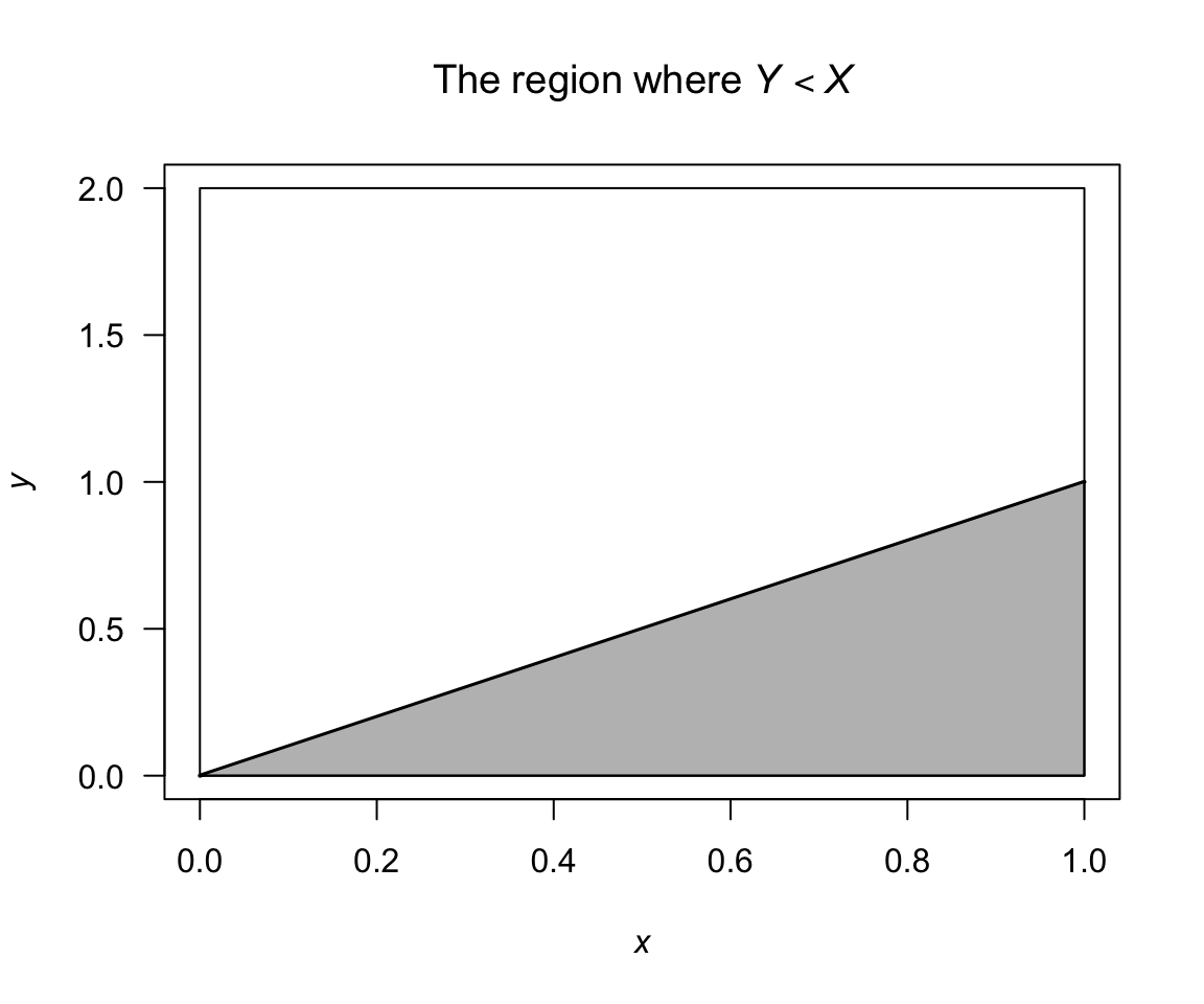
FIGURE 6.3: The region where $Y < X$

Example 6.11 (Bivariate discrete marginal distributions) Recall Example 6.5, where two dice are rolled. We can find the marginal distributions of $X$ and $Y$ (Table 6.5). The probabilities in the first row (where $Y = 0$), for instance, are summed and appear as the first term in the final column; this is the marginal distribution for $Y = 0$. Similarly for the other rows.

Recalling that $X$ is the number of times a is rolled when two dice are thrown, the distribution of $X$ should be $\text{Bin}(2, 1/6$); the probabilities given in the last row of the table agree with this. That is, $\Pr(X = x) = \binom{2}{x}\left(\frac{1}{6}\right)^x \left(\frac{5}{6}\right)^{2 - x}$ for $x = 0, 1, 2$. Of course, the distribution of $Y$ is the same.

TABLE 6.5: The marginal distributions

	$x = 0$	$x = 1$	$x = 2$	$\Pr(Y = y)$
$y = 0$	$4/9$	$2/9$	$1/36$	$25/36$
$y = 1$	$2/9$	$1/18$	$0$	$10/36$
$y = 2$	$1/36$	$0$	$0$	$1/36$
$\Pr(X = x)$	$25/36$	$10/36$	$1/36$	$1$

Example 6.12 (Bivariate discrete marginal distributions) Consider again the random process in Example 6.8. From Table 6.2, the marginal distribution for $X_1$ is found simply by summing over the values for $X_2$ in the table. When $x_1 = 0$, $$p_{X_1}(0) = \sum_{x_2} p_{X_1, X_2}(0,x_2) = 1/24 + 1/24 + 1/24 +\dots = 6/24.$$ Likewise, $$\begin{align*} p_{X_1}(1) &= \sum_{x_2} p_{X_1, X_2}(1,x_2) = 6/12;\\ p_{X_1}(2) &= \sum_{x_2} p_{X_1, X_2}(2,x_2) = 6/24. \end{align*}$$ So the marginal distribution of $X_1$ is $$p_{X_1}(x_1) = \begin{cases} 1/4 & \text{if $x_1 = 0$};\\ 1/2 & \text{if $x_1 = 1$};\\ 1/4 & \text{if $x_1 = 2$};\\ 0 & \text{otherwise}.\\ \end{cases}$$ This is equivalent to adding the row probabilities in Table 6.2. In this example, the marginal distribution is easily found from the total column of Table 6.2.

6.2.4 Conditional distributions

Consider $(X, Y)$ with joint probability function as in Example 6.2, with marginal distributions of $X$ and $Y$ as shown in Table 6.6.

TABLE 6.6: A joint distribution with the marginal distributions

	$x = 0$	$x = 1$	$x = 2$	$\Pr(Y = y)$
$y = 0$	$1/36$	$1/6$	$1/4$	$4/9$
$y = 1$	$1/9$	$1/3$	$0$	$4/9$
$y = 2$	$1/9$	$0$	$0$	$1/9$
$\Pr(X = x)$	$1/4$	$1/2$	$1/4$	$1$

Suppose we want to evaluate the conditional probability $\Pr(X = 1 \mid Y = 1)$. We use that $\Pr(A \mid B) = \Pr(A \cap B)/\Pr(B)$. So $$\Pr(X = 1 \mid Y = 1) = \frac{\Pr(X = 1, Y = 1)}{\Pr(Y = 1)} = \frac{1/3}{4/9} = \frac{3}{4}.$$ So, for each $x\in R_X$ we could find $\Pr(X = x, Y = 1)$ and this is then the conditional distribution of $X$ given that $Y = 1$.

Definition 6.7 (Bivariate discrete conditional distributions) For a discrete random vector $(X, Y)$ with probability function $p_{X, Y}(x, y)$ the conditional probability distribution of $X$ given $Y = y$ is defined by
$$\begin{align} p_{X \mid Y = y}(x \mid y) &= \Pr(X = x \mid Y = y)\\ &= \frac{\Pr(X = x, Y = y)}{\Pr(Y = y)}\\ &= \frac{p_{X, Y}(x, y)}{p_Y(y)} \end{align}$$ for $x \in R_X$ and provided $p_Y(y) > 0$.

The continuous case is analagous.

Definition 6.8 (Bivariate continuous marginal distributions) If $(X, Y)$ is a continuous 2-dimensional random variable with joint pdf $f_{X, Y}(x, y)$ and respective marginal pdfs $f_X(x)$, $f_Y(y)$, then the conditional probability distribution of $X$ given $Y = y$ is defined by
$$\begin{equation} f_{X \mid Y = y}(x \mid y) = \frac{f_{X, Y}(x, y)}{f_Y(y)} \end{equation}$$ for $x \in R_X$ and provided $f_Y(y) > 0$.

The above conditional pdfs satisfy the requirements for a univariate pdf; that is, $f_{X \mid Y}(x \mid y) \ge 0$ for all $x$ and $\int_0^\infty f_{X\mid Y}(x\mid y)\,dx = 1$.

Example 6.13 (Bivariate continuous marginal distributions) In Example 6.10, the joint pdf of $X$ and $Y$ considered was $$f_{X,Y}(x,y) = \begin{cases} \frac{1}{3}(3x^2 + xy) & \text{for $0 \leq x \leq 1$ and $0 \leq y \leq 2$};\\ 0 & \text{elsewhere}. \end{cases}$$ The marginal pdfs of $X$ and $Y$ are $$\begin{align*} f_X(x) &= 2x^2 + \frac{2}{3}x \quad\text{for $0 \leq x \leq 1$}; \\ f_Y(y) &= \frac{1}{6}(2 + y) \quad \text{for $0 \leq y \leq 2$}. \end{align*}$$ Hence, the conditional distribution of $X \mid Y = y$ is $$f_{X\mid Y = y}(x \mid y) = \frac{(3x^2 + xy)/3}{(2 + y)/6} = \frac{2x(3x + y)}{2 + y} \quad\text{for $0 \leq x \leq 1$},$$ and the conditional distribution of $Y \mid X = x$ is $$f_{Y \mid X = x}(y \mid x) = \frac{3x + y}{2(3x + 1)}\quad\text{for $0 \leq y \leq 2$}.$$ Both these conditional density functions are valid density functions (verify!).

The marginal distribution for $Y$, and two conditional distributions of $Y$ (given $X = 0.1$ and $X = 0.9$) are shown in Fig. 6.4.

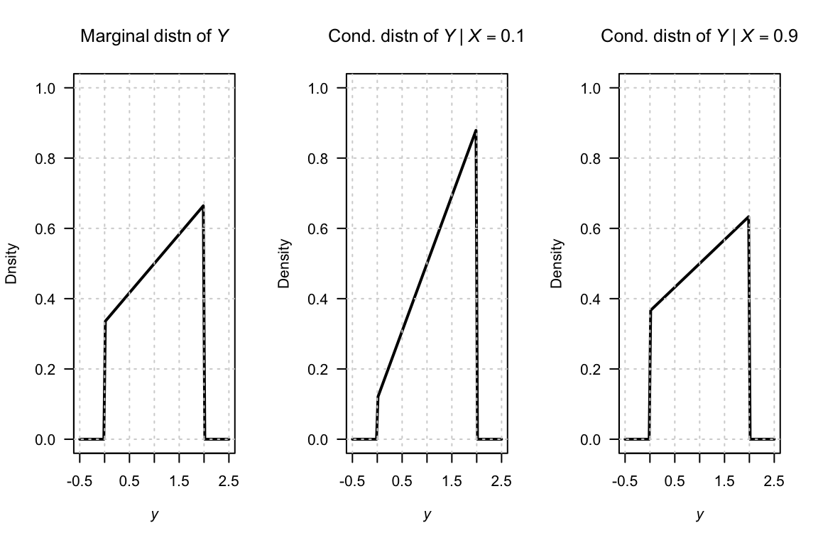
FIGURE 6.4: The marginal distribution of $Y$ (left panel), and the conditional distribution of $Y$ for $X = 0$ (centre panel) and $X = 1$ (right panel).

To interpret the conditional distribution, for example $f_{X \mid Y = y}(x \mid y)$, consider slicing through the surface $f_{X, Y}(x, y)$ with the plane $y = c$ say, for $c$ a constant (see below). The intersection of the plane with the surface, will be proportional to a $1$-dimensional pdf. This is $f_{X, Y}(x, c)$, which will not, in general, be a density function since the area under this curve will be $f_Y(c)$. Dividing by the constant $f_Y(c)$ ensures the area under $\displaystyle\frac{f_{X,Y}(x,c)}{f_Y(c)}$ is one. This is a one-dimensional pdf, of $X$ given $Y = c$; that is $f_{X \mid Y = c}(x\mid c)$.

FIGURE 6.5: A bivariate distribution

FIGURE 6.6: A bivariate distribution, sliced at $Y = 1$, showing the conditional distribution of $X$ when $Y = 0.5$

Example 6.14 (Bivariate discrete conditional distributions) Consider again the random process in Example 6.4. The conditional distribution for $X_2$ given $X_1 = 0$ can be found from Table 6.6. First, $p_{X_1}(x_1)$, is needed, which was done in Example 6.12. Then,

$$\begin{align*} p_{X_2\mid X_1 = 0}(x_2\mid X_1 = 0) &= \frac{p_{X_1, X_2}(0, x_2)}{p_{X_1}(0)} \\ &= \frac{p_{X_1, X_2}(0, x_2)}{1/4}, \end{align*}$$ from which we can deduce $$p_{X_2 \mid X_1 = 0}(x_2 \mid X_1 = 0) = \begin{cases} \frac{1/24}{1/4} = 1/6 & \text{for $x_2 = 1$};\\ \frac{1/24}{1/4} = 1/6 & \text{for $x_2 = 2$};\\ \frac{1/24}{1/4} = 1/6 & \text{for $x_2 = 3$};\\ \frac{1/24}{1/4} = 1/6 & \text{for $x_2 = 4$};\\ \frac{1/24}{1/4} = 1/6 & \text{for $x_2 = 5$};\\ \frac{1/24}{1/4} = 1/6 & \text{for $x_2 = 6$}.\\ \end{cases}$$ The conditional distribution $p_{X_2\mid X_1 = x_1}(x_2\mid x_1)$ is a probability function for $X_2$ (verify!). Since $X_2$ was the number of the top face of the die, this is exactly as we should expect.

6.3 Independent random variables

Recall that events $A$ and $B$ are independent if, and only if, $$\Pr(A \cap B) = \Pr(A)\Pr(B).$$ An analogous definition applies for random variables.

Definition 6.9 (Independent random variables) The random variables $X$ and $Y$ with joint df $F_{X, Y}$ and marginal dfs $F_X$ and $F_Y$ are independent if, and only if, $$\begin{equation} F_{X, Y}(x, y) = F_X(x) \times F_Y(y) \end{equation}$$ for all $x$ and $y$.

If $X$ and $Y$ are not independent they are dependent, or not independent.

The following theorem is often used to establish independence or dependence of random variables. The proof is omitted.

Theorem 6.1 The discrete random variables $X$ and $Y$ with joint probability function $p_{X, Y}(x, y)$ and marginals $p_X(x)$ and $p_Y(y)$ are independent if, and only if,

$$\begin{equation} p_{X, Y}(x, y) = p_X(x) \times p_Y(y) \text{ for every }(x, y) \in R_{X \times Y}. \tag{6.5} \end{equation}$$ The continuous random variables $(X, Y)$ with joint pdf $f_{X, Y}$ and marginal pdfs $f_X$ and $f_Y$ are independent if, and only if,

$$\begin{equation} f_{X, Y}(x, y) = f_X(x)\times f_Y(y) \end{equation}$$ for all $x$ and $y$.

To show independence for continuous random variables (and analogously for discrete random variables) we must show $f_{X, Y}(x, y) = f_X(x)\times f_Y(y)$ for all pairs $(x, y)$. If $f_{X, Y}(x, y)\neq f_X(x)\times f_Y(y)$, even for any one particular pair of $(x, y)$, then $X$ and $Y$ are dependent.

Example 6.15 (Bivariate discrete: Independence) The random variables $X$ and $Y$ have the joint probability distribution shown in Table 6.7. Summing across rows, the marginal probability function of $Y$ is: $$p_Y(y) = \begin{cases} 1/6 & \text{for $y = 1$};\\ 1/3 & \text{for $y = 2$};\\ 1/2 & \text{for $y = 3$}. \end{cases}$$ To determine if $X$ and $Y$ are independent, the marginal probability function of $X$ is also needed: $$p_X(x) = \begin{cases} 1/5 & \text{for $x = 1$};\\ 1/5 & \text{for $x = 2$};\\ 2/5 & \text{for $x = 3$};\\ 1/5 & \text{for $x = 4$}. \end{cases}$$ Clearly (6.5) is satisfied for all pairs $(x, y)$, so $X$ and $Y$ are independent.

TABLE 6.7: A joint pf

	$x = 1$	$x = 2$	$x = 3$	$x = 4$
$y = 1$	$1/30$	$1/30$	$2/30$	$1/30$
$y = 2$	$2/30$	$2/30$	$4/30$	$2/30$
$y = 3$	$3/30$	$3/30$	$6/30$	$3/30$

Example 6.16 (Bivariate continuous: Independence) Consider the random variables $X$ and $Y$ with joint pdf $$f(x, y) = \begin{cases} 4xy & \text{for $0 < x < 1$ and $0 < y < 1 $}\\ 0 & \text{elsewhere}.\\ \end{cases}$$ To show that $X$ and $Y$ are independent, the marginal distributions of $X$ and $Y$ are needed. Now $$f_X(x) = \int_0^1 4xy \, dy = 2x\quad\text{for $0 < x < 1$}.$$ Similarly $f_Y(y) = 2y$ for $0 < y < 1$. Thus we have $f_X(x) \, f_Y(y) = f(x,y)$, so $X$ and $Y$ are independent.

Example 6.17 (Bivariate discrete: Independence) Consider again the random process in Example 6.4. The marginal distribution of $X_1$ was found in Example 6.12. The marginal distribution of $X_2$ is (check!) $$p_{X_2}(x_2) = \begin{cases} \frac{1/24}{1/4} = 1/6 & \text{for $x_2 = 1$};\\ \frac{1/24}{1/4} = 1/6 & \text{for $x_2 = 2$};\\ \frac{1/24}{1/4} = 1/6 & \text{for $x_2 = 3$};\\ \frac{1/24}{1/4} = 1/6 & \text{for $x_2 = 4$};\\ \frac{1/24}{1/4} = 1/6 & \text{for $x_2 = 5$};\\ \frac{1/24}{1/4} = 1/6 & \text{for $x_2 = 6$}.\\ \end{cases}$$ To determine if $X_1$ and $X_2$ are independent, each $x_1$ and $x_2$ pair must be considered. As an example, we see $$\begin{align*} p_{X_1}(0) \times p_{X_2}(1) = 1/4 \times 1/6 = 1/24 &= p_{X_1, X_2}(0, 1);\\ p_{X_1}(0) \times p_{X_2}(2) = 1/4 \times 1/6 = 1/24 &= p_{X_1, X_2}(0, 2);\\ p_{X_1}(1) \times p_{X_2}(1) = 1/2 \times 1/6 = 1/12 &= p_{X_1, X_2}(1, 1);\\ p_{X_1}(2) \times p_{X_2}(1) = 1/4 \times 1/6 = 1/24 &= p_{X_1, X_2}(2, 1). \end{align*}$$ This is true for all pairs, and so $X_1$ and $X_2$ are independent random variables. Independence is, however, obvious from the description of the random process (Example 6.1), and is easily seen from Table 6.2.

Example 6.18 (Bivariate continuous: Independence) Consider the continuous random variables $X_1$ and $X_2$ with joint pdf $$f_{X_1, X_2}(x_1, x_2) = \begin{cases} \frac{2}{7}(x_1 + 2x_2) & \text{for $0 < x_1 < 1$ and $1 < x_2 < 2$};\\ 0 & \text{elsewhere.} \end{cases}$$ The marginal distribution of $X_1$ is $$f_{X_1}(x_1) = \int_1^2 \frac{2}{7}(x_1 + 2x_2)\,dx_2\\ = \frac{2}{7}(x_1 + 3)$$ for $0 < x_1 < 1$ (and zero elsewhere). Likewise, the marginal distribution of $X_2$ is $$f_{X_2}(x_2) = \frac{2}{7}(x_1^2/2 + 2 x_1 x_2)\Big|_{x_1 = 0}^1 = \frac{1}{7}(1 + 4x_2)$$ for $1 < x_2 < 2$ (and zero elsewhere). (Both the marginal distributions must be valid density functions; verify!) Since $$f_{X_1}(x_1) \times f_{X_2}(x_2) = \frac{2}{49}(x_1 + 3)(1 + 4x_2) \ne f_{X_1, X_2}(x_1, x_2),$$ the random variables $X_1$ and $X_2$ are not independent.

The conditional distribution of $X_1$ given $X_2 = x_2$ is $$\begin{align*} f_{X_1 \mid X_2 = x_2}(x_1 \mid x_2) &= \frac{ f_{X_1, X_2}(x_1, x_2)}{ f_{X_2}(x_2)} \\ &= \frac{ (2/7) (x_1 + 2x_2)}{ (1/7)(1 + 4x_2)} \end{align*}$$ for $0 < x_1 < 1$ and any given value of $1 < x_2 < 2$. (Again, this conditional density must be a valid pdf.) So, for example, $$f_{X_1 \mid X_2 = 1.5}(x_1\mid x_2 = 1.5) = \frac{ (2/7) (x_1 + 2\times 1.5)}{ (1/7)(1 + 4\times 1.5)} = \frac{2}{7}(x_1 + 3)$$ for $0 < x_1 < 1$ and is zero elsewhere. And, $$f_{X_1\mid X_2 = 1}(x_1 \mid 1) = \frac{ (2/7) (x_1 + 2\times 1)}{ (1/7)(1 + 4\times 1)} = \frac{2}{5}(x_1 + 2)$$ for $0 < x_1 < 1$ and is zero elsewhere. Since the distribution of $X_1$ depends on the given value of $X_2$, $X_1$ and $X_2$ are not independent.

Example 6.19 (Bivariate continuous: Independence) Consider the two continuous random variables $Y_1$ and $Y_2$ with joint pf $$f_{Y_1, Y_2}(y_1, y_2)= \begin{cases} 2(y_1 + y_2) & \text{for $0 < y_1 < y_2 < 1$};\\ 0 & \text{elsewhere}. \end{cases}$$ A diagram of the region over which $Y_1$ and $Y_2$ are defined is shown in Fig. 6.7. To determine if $Y_1$ and $Y_2$ are independent, the two marginal distributions are needed. For example: $$f_{Y_1}(y_1) = 1 + 2y_1 - 3y_1^2\quad\text{for $0 < y_1 < 1$}.$$ Since the distribution of $Y_1$ depends on the value of $Y_2$, then $Y_1$ and $Y_2$ are not independent.

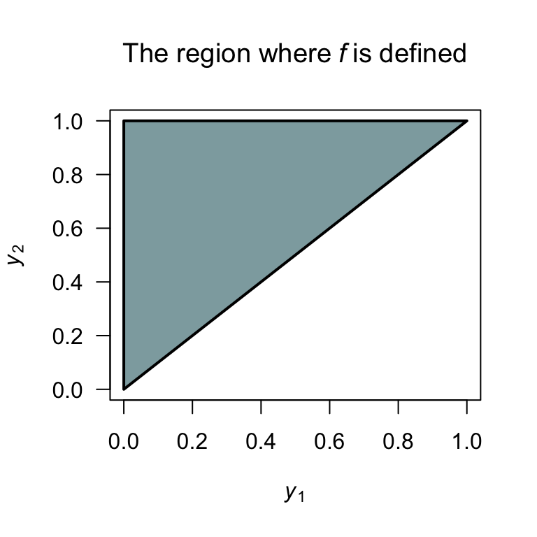
FIGURE 6.7: The region over which $f_{Y_1, Y_2}(y_1, y_2)$ is defined

6.4 Expectations

6.4.1 Expectations for bivariate distributions

In a manner analogous to the univariate case, the expectation of functions of two random variables can be given.

Definition 6.10 (Expectation for bivariate distributions) Let $(X, Y)$ be a 2-dimensional random variable and let $u(X, Y)$ be a function of $X$ and $Y$. Then the expectation or expected value of $\text{E}[u(X, Y)]$ is

• $\displaystyle \text{E}[u(X, Y)] = \sum\sum_{(x, y)\in R}u(x, y) p_{X, Y}(x, y)$ for $(X, Y)$ discrete with probability function $p_{X, Y}(x, y)$ for $(x, y) \in R$;

• $\displaystyle \text{E}[(u(X, Y)] = \int \!\!\int_R u(x, y) f_{X, Y}(x, y) \, dx \, dy$ for $(X, Y)$ continuous with pdf $f_{X, Y}(x, y)$ for $(x, y) \in R$.

This definition can be extended to the expectation of a function of any number of random variables.

Example 6.20 (Expectation of function of two rvs (discrete)) Consider the joint distribution of $X$ and $Y$ in Example 6.4. Determine $\text{E}(X + Y)$; i.e., the mean of the number of heads plus the number showing on the die.

From the Definition 6.10, write $u(X, Y) = X + Y$ and so

$$\begin{align*} \text{E}(X + Y) &= \sum_{x = 0}^2 \sum_{y = 1}^6 (x + y) p_{X, Y}(x, y)\\ &= 1\times(1/24) + 2\times(1/24) + \dots + 6\times(1/24)\\ & \qquad + 2\times(1/12) + 3\times(1/12) + \dots + 7\times(1/12)\\ & \qquad + 3\times(1/24) + 4\times(1/24) + \dots + 8\times(1/24)\\ &= 21/24 + 27/12 + 33/24\\ &= 4.5. \end{align*}$$ The answer is just $\text{E}(X) + \text{E}(Y) = 1 + 3.5 = 4.5$. This is no coincidence, as we see from Theorem 6.2.

Example 6.21 (Expectation of function of two rvs (continuous)) Consider Example 6.6. To determine $\text{E}(XY)$, write $u(X, Y) = XY$ and proceed: $$\text{E}(XY) = \frac{6}{5} \int_0^1\int_0^1 xy(x + y^2)\,dx\,dy = \frac7{20}.$$ Unlike the previous example, an alternative simple calculation based on $\text{E}(X)$ and $\text{E}(Y)$ is not possible, since $\text{E}(XY)\neq\text{E}(X) \text{E}(Y)$ in general.

Theorem 6.2 (Expectations of two rvs) If $X$ and $Y$ are any random variables and $a$ and $b$ are any constants then $$\text{E}(aX + bY) = a\text{E}(X) + b\text{E}(Y).$$

This theorem is no surprise after seeing Theorem 3.1, but is powerful and useful. The proof given here is for the discrete case; the continuous case is analogous.

Proof. $$\begin{align*} E(aX + bY) &= \sum\sum_{(x, y) \in R}(ax + by) \, p_{X, Y}(x, y), \text{ by definition}\\ &= \sum_x \sum_y ax p_{X, Y}(x, y) + \sum_x \sum_y by p_{X, Y}(x, y)\\ &= a\sum_x x\sum_y p_{X, Y}(x, y) + b\sum_y y\sum_x p_{X, Y}(x, y)\\ &= a\sum_x x \Pr(X = x) + b\sum_y y \Pr(Y = y)\\ &= a\text{E}(X) + b\text{E}(Y). \end{align*}$$

This result is true whether or not $X$ and $Y$ are independent. Theorem 6.2 naturally generalises to the expected value of a linear combination of random variables (see Theorem 6.5).

6.4.2 Moments of a bivariate distribution: Covariance

The idea of a moment in the univariate case naturally extends to the bivariate case. Hence, define $\mu'_{rs} = \text{E}(X^r Y^s)$ or $\mu_{rs} = \text{E}\big((X - \mu_X)^r (Y - \mu_Y)^s\big)$ as the raw and central moments for a bivariate distribution.

The most important of these moments is the covariance.

Definition 6.11 (Covariance) The covariance of $X$ and $Y$ is defined as $$\begin{align*} \text{Cov}(X, Y) &= \text{E}[(X - \mu_X)(Y - \mu_Y)]\\ &= \begin{cases} \displaystyle \sum_{x} \sum_{y} (x - \mu_X)(y - \mu_Y) p_{X, Y}(x, y) & \text{for $X, Y$ discrete};\\[6pt] \displaystyle \int_{-\infty}^\infty\!\int_{-\infty}^\infty (x - \mu_X)(y - \mu_Y) f_{X, Y}(x, y)\, dx\, dy & \text{for $X, Y$ continuous}. \end{cases} \end{align*}$$

The covariance is a measure of how $X$ and $Y$ vary jointly, in the sense that a positive covariance indicates that ‘on average’ $X$ and $Y$ increase (or decrease) together whereas a negative covariance indicates that `on average’ as $X$ increases and $Y$ decreases (and vice versa). We say that covariance is a measure of linear dependence.

Covariance is best evaluated from the computational formula:

Theorem 6.3 (Covariance) For any random variables $X$ and $Y$, $$\text{Cov}(X, Y) = \text{E}(XY) - \text{E}(X)\text{E}(Y).$$

Proof. The proof uses Theorems 3.1 and 6.2. $$\begin{align*} \text{Cov}(X, Y) &= \text{E}\big( (X - \mu_X)(Y-\mu_Y)\big) \\ &= \text{E}( XY - \mu_X Y - \mu_Y X+ \mu_X\mu_Y) \\ &= \text{E}( XY ) - \mu_X\text{E}(Y) - \mu_Y\text{E}(X) + \mu_X \mu_Y \\ &= \text{E}( XY ) - \mu_X\mu_Y - \mu_Y\mu_X + \mu_X \mu_Y \\ &= \text{E}( XY ) - \mu_X \mu_Y. \end{align*}$$

Computing the covariance is tedious: $\text{E}(X)$, $\text{E}(Y)$, $\text{E}(X Y)$ need to be computed, and so the joint and marginal distributions of $X$ and $Y$ are needed.

Covariance has units given by the product of the units of $X$ and $Y$. For example, if $X$ is in metres and $Y$ is in seconds then $\text{Cov}(XY)$ has the units metre-seconds. To compare the strength of covariation amongst pairs of random variables, a unitless measure is useful. Correlation does this by scaling the covariance in terms of the standard deviations of the individual variables.

Definition 6.12 (Correlation) The correlation coefficient between the random variables $X$ and $Y$ is denoted by $\text{Corr}(X, Y)$ or $\rho_{X, Y}$ and is defined as $$\rho_{X, Y} = \frac{\text{Cov}(X, Y)}{\sqrt{ \text{var}(X)\text{var}(Y)}} = \frac{\sigma_{X, Y}}{\sigma_X \sigma_Y}.$$

If there is no confusion over which random variables are involved, we write $\rho$ rather than $\rho_{XY}$. It can be shown that $-1 \leq \rho \leq 1$.

Example 6.22 (Correlation coefficient (discrete rvs)) Consider two discrete random variables $X$ and $Y$ with the joint pf given in Table 6.8. To compute the correlation coefficient, the following steps are required.

• $\text{Corr}(X, Y) = \text{Cov}(X, Y)/\sqrt{ \text{var}(X)\text{var}(Y) }$, so $\text{var}(X)$, $\text{var}(Y)$ must be computed;
• To find $\text{var}(X)$ and $\text{var}(Y)$, $\text{E}(X)$ and $\text{E}(X^2)$, $\text{E}(Y)$ and $\text{E}(Y^2)$ are needed, so the marginal pfs of $X$ and $Y$ are needed.

So first, the marginal pfs are $$p_X(x) = \sum_{y = -1, 1} p_{X, Y}(x, y) = \begin{cases} 7/24 & \text{for $x = 0$};\\ 8/24 & \text{for $x = 1$};\\ 9/24 & \text{for $x = 2$};\\ 0 & \text{otherwise} \end{cases}$$ and $$p_Y(y) = \sum_{x = 0}^2 p_{X, Y}(x, y) = \begin{cases} 1/2 & \text{for $y = -1$};\\ 1/2 & \text{for $y = 1$};\\ 0 & \text{otherwise.} \end{cases}$$ Then, $$\begin{align*} \text{E}(X) &= (7/24 \times 0) + (8/24 \times 1) + (9/24\times 2) = 26/24;\\ \text{E}(X^2) &= (7/24 \times 0^2) + (8/24 \times 1^2) + (9/24\times 2^2) = 44/24;\\ \text{E}(Y) &= (1/2 \times -1) + (1/2 \times 1) = 0;\\ \text{E}(Y^2) &= (1/2 \times (-1)^2) + (1/2 \times 1^2) = 1, \end{align*}$$ giving $\text{var}(X) = 44/24 - (26/24)^2 = 0.6597222$ and $\text{var}(Y) = 1 - 0^2 = 1$. Then, $$\begin{align*} \text{E}(XY) &= \sum_x\sum_y xy\,p_{X,Y}(x,y) \\ &= (0\times -1 \times 1/8) + (0\times 1 \times 1/6) + \cdots + (2\times 1 \times 1/4) \\ &= 1/12. \end{align*}$$ Hence, $$\text{Cov}(X,Y) = \text{E}(XY) - \text{E}(X) \text{E}(Y) = \frac{1}{12} - \left(\frac{26}{24}\times 0\right) = 1/12,$$ and $$\text{Corr}(X,Y) = \frac{ \text{Cov}(X,Y)}{\sqrt{ \text{var}(X)\text{var}(Y) } } = \frac{1/12}{\sqrt{0.6597222 \times 1}} = 0.1025978,$$ so the correlation coefficient is about $0.10$, and a small positive linear association exists between $X$ and $Y$.

TABLE 6.8: A bivariate discrete probability function

	$x = 0$	$x = 1$	$x = 2$	Total
$y = 1$	$1/30$	$1/30$	$2/30$	$1/30$
$y = 2$	$2/30$	$2/30$	$4/30$	$2/30$
$y = 3$	$3/30$	$3/30$	$6/30$	$3/30$

6.4.3 Properties of covariance and correlation

• The correlation has no units.
• The covariance has units; if $X_1$ is measured in kilograms and $X_2$ in centimetres, then the units of the covariance are kg-cm.
• If the units of measurements change, the numerical value of the covariance changes, but the numerical value of the correlation stays the same. (For example, if $X_1$ is changed from kilograms to grams, the numerical value of the correlation will not change in value, but the numerical values of covariance will change.)
• The correlation is a number between $-1$ and $1$ (inclusive). When the correlation coefficient (or covariance) is negative, a negative linear relationship is said to exist between the two variables. Likewise, when the correlation coefficient (or covariance) is positive, a positive linear relationship is said to exist between the two variables.
• When the correlation coefficient (or covariance) is zero, no linear dependence is said to exist.

Theorem 6.4 (Properties of the covariance) For random variables $X$, $X$ and $Z$, and constants $a$ and $b$:

• $\text{Cov}(X, Y) = \text{Cov}(Y, X)$.
• $\text{Cov}(aX,bY) = ab\,\text{Cov}(X, Y)$.
• $\text{var}(aX + bY) = a^2\text{var}(X) + b^2\text{var}(Y) + ab\,\text{Cov}(X, Y)$.
• If $X$ and $Y$ are independent, then $\text{E}(X Y) = \text{E}(X)\text{E}(Y)$ and hence $\text{Cov}(X,Y) = 0$.
• $\text{Cov}(X, Y) = 0$ does not imply $X$ and $Y$ are independent, except for the special case of the bivariate normal distribution.

A zero correlation coefficient in an indication of no linear dependence only. A relationship may still exist between $X$ and $Y$ even if the correlation is zero.

Example 6.23 (Linear dependence and correlation) Consider $X_1$ with the pf:

$x_1$	$-1$	$0$	$1$
$p_{X_1}(x_1)$	$1/3$	$1/3$	$1/3$

Then, define $X_2$ to be explicitly related to $X_1$: $X_2 = X_1^2$. So, we know a relationship exists between $X_1$ and $X_2$ (but it is not linear). The joint pf for $(X_1, X_2)$ is shown in Table 6.9.å Then

$$\begin{equation*} \text{Cov}(X_1, X_2) = \text{E}(X_1 X_2) - \text{E}(X_1)\text{E}(X_2) = 0 - 0\times 2/3 = 0 \end{equation*}$$ so $\text{Corr}(X_1, X_2) = 0$. But $X_1$ and $X_2$ are certainly related as $X_2$ was explicitly defined as a function of $X_1$.

Since the correlation is a measure of the strength of the linear relationship between two random variables, a correlation of zero simply is indication of no linear relationship between $X_1$ and $X_2$. (As is the case in this example, there may be a different relationship between the variables, but no linear relationship.)

TABLE 6.9: A bivariate discrete probability function

	$x_1 = -1$	$x_1 = 0$	$x_1 = 1$	Total
$x_2 = 0$	$0$	$1/3$	$0$	$1/3$
$x_2 = 1$	$1/3$	$0$	$1/3$	$2/3$
Total	$1/3$	$1/3$	$1/3$	$1$

6.5 Conditional expectations

Conditional expectations are simply expectations computed from a conditional distribution.

6.5.1 Conditional mean

The conditional mean is the expected value computed from a conditional distribution.

Definition 6.13 (Conditional expectation) The conditional expected value or conditional mean of a random variable $X$ for given $Y = y$ is denoted by $\text{E}(X \mid Y = y)$ and is defined as

$$\begin{align*} \text{E}(X \mid Y = y) &= \begin{cases} \displaystyle \sum_{x} x p_{X\mid Y}(x\mid y) & \text{if $p_{X\mid Y}(x\mid y)$ is the conditional pf};\\[6pt] \displaystyle \int_{-\infty}^\infty x f_{X\mid Y}(x\mid y)\, dx & \text{if $f_{X\mid Y}(x\mid y)$ is the conditional pdf}.\\ \end{cases} \end{align*}$$

$\text{E}(X \mid Y = y)$ is typically denoted $\mu_{X \mid Y = y}$.

Example 6.24 (Conditional mean (continuous)) Consider the two random variables $X$ and $Y$ with joint pdf $$f_{X, Y}(x, y) = \begin{cases} \frac{3}{5}(x + xy + y^2) & \text{for $0 < x < 1$ and $-1 < y < 1$};\\ 0 & \text{otherwise.} \end{cases}$$ To find $f_{Y \mid X = x}(y\mid x)$, first $f_X(x)$ is needed: $$f_X(x) = \int_{-1}^1 f_{X,Y}(x,y) dy = \frac{3}{15}(6x + 2)$$ for $0 < x < 1$. Then, $$f_{Y \mid X = x}(y \mid x) = \frac{ f_{X, Y}(x, y)}{ f_X(x) } = \frac{3(x + xy + y^2)}{6x + 2}$$ for $-1 < y < 1$ and given $0 < x < 1$. The expected value of $Y$ given $X = x$ is then $$\text{E}(Y\mid X = x) = \frac{x}{3x + 1}.$$ This expression indicates that the conditional expected value of $Y$ depends on the given value of $X$; for example, $$\begin{align*} \text{E}(Y\mid X = 0) &= 0;\\ \text{E}(Y\mid X = 0.5) &= 0.2;\\ \text{E}(Y\mid X = 1) &= 1/4. \end{align*}$$ Since $\text{E}(Y\mid X = x)$ depends on the value of $X$, $X$ and $Y$ are not independent.

6.5.2 Conditional variance

The conditional variance is the variance computed from a conditional distribution.

Definition 6.14 (Conditional variance) The conditional variance of a random variable $X$ for given $Y = y$ is denoted by $\text{var}(X \mid Y = y)$ and is defined as

$$\begin{align*} \text{var}(X \mid Y = y) &= \begin{cases} \displaystyle \sum_{x} (x-\mu_{X\mid y})^2 p(x\mid y) & \text{if $p(x\mid y)$ is the conditional pf};\\[6pt] \displaystyle \int_{-\infty}^\infty (x-\mu_{X\mid y})^2 f(x\mid y)\, dx & \text{if $f(x\mid y)$ is the conditional pdf}.\\ \end{cases} \end{align*}$$ where $\mu_{X \mid y}$ is the conditional mean of $X$ given $Y = y$.

$\text{var}(X \mid Y = y)$ is typically denoted $\sigma^2_{X \mid Y = y}$.

Example 6.25 (Conditional variance (continuous)) Refer to Example 6.24. The conditional variance of $Y$ given $X = x$ can be found by first computing $\text{E}(Y^2\mid X = x)$.

$$\begin{align*} \text{E}(Y^2\mid X = x) &= \int_{-1}^1 y^2 f_{Y\mid X = x}(y\mid x)\,dy \\ &= \frac{3}{6x + 2} \int_{-1}^1 y^2 (x + xy + y^2)\, dy \\ &= \frac{5x + 3}{5(3x + 1)}. \end{align*}$$ So the conditional variance is

$$\begin{align*} \text{var}(Y\mid X = x) &= \text{E}(Y^2\mid X = x) - \left( \text{E}(Y\mid X = x) \right)^2 \\ &= \frac{5x+3}{5(3x + 1)} - \left( \frac{x}{3x + 1}\right)^2 \\ &= \frac{10x^2 + 14x + 3}{5(3x + 1)^2} \end{align*}$$ for given $0 < x < 1$. Hence the variance of $Y$ depends on the value of $X$ that is given; for example,

$$\begin{align*} \text{var}(Y\mid X = 0) &= 3/5 = 0.6\\ \text{var}(Y\mid X = 0.5) &= \frac{10\times (0.5)^2 + (14\times0.5) + 3}{5(3\times0.5 + 1)^2} = 0.4\\ \text{var}(Y\mid X = 1) &= 27/80 = 0.3375. \end{align*}$$

In general, to compute the conditional variance of $X\mid Y = y$ given a joint probability function, the following steps are required.

• Find the marginal distribution of $Y$.
• Use this to compute the conditional probability function $f_{X \mid Y = y}(x \mid y) = f_{X, Y}(x, y)/f_{X}(x)$.
• Find the conditional mean $\text{E}(X \mid Y = y)$.
• Find the conditional second raw moment $\text{E}(X^2 \mid Y = y)$.
• Finally, compute $\text{var}(X\mid Y=y) = \text{E}(X^2\mid Y=y) - (\text{E}(X\mid Y=y))^2$.

Example 6.26 (Conditional variance (discrete)) Two discrete random variables $U$ and $V$ have the joint pf given in Table 6.10. To find the conditional variance of $V$ given $U = 11$, use the steps above.

1. First, find the marginal distribution of $U$: $$p_U(u) = \begin{cases} 4/9 & \text{for $u = 10$};\\ 7/18 & \text{for $u = 11$};\\ 1/6 & \text{for $u = 12$};\\ 0 & \text{otherwise.}\\ \end{cases}$$

2. Secondly, compute the conditional probability function: $$\begin{align*} p_{V\mid U = 11}(v \mid u = 11) &= p_{U, V}(u,v)/p_{U}(u = 11) \\ &= \begin{cases} \frac{1/18}{7/18} = 1/7 & \text{if $v = 0$};\\ \frac{1/3}{7/18} = 6/7 & \text{if $v = 1$} \end{cases} \end{align*}$$ using $p_U(u = 11) = 7/18$ from the Step 1.

3. Thirdly, find the conditional mean: $$\text{E}(V\mid U = 11) = \sum_v v p_{V\mid U = 11}(v\mid u) = \left(\frac{1}{7}\times 0\right) + \left(\frac{6}{7}\times 1\right) = 6/7.$$

4. Fourthly, find the conditional second raw moment: $$\text{E}(V^2\mid U = 11) = \sum_v v^2 p_{V\mid U = 11}(v\mid u) = \left(\frac{1}{7}\times 0^2\right) + \left(\frac{6}{7}\times 1^2\right) = 6/7.$$

5. Finally, compute: $$\begin{align*} \text{var}(V\mid U = 11) &= \text{E}(V\mid U = 11) - (\text{E}(V\mid U = 11))^2\\ &= (6/7) - (6/7)^2\\ &\approx 0.1224. \end{align*}$$

TABLE 6.10: A bivariate discrete probability function

	$u = 10$	$u = 11$	$u = 12$	Total
$v = 0$	$1/9$	$1/18$	$1/6$	$1/3$
$v = 1$	$1/3$	$1/3$	$0$	$2/3$
Total	$4/9$	$7/18$	$1/6$	$1$

6.6 The multivariate extension

6.6.1 Expectation

Results involving expectations naturally generalise from the bivariate to the multivariate case. Firstly, the expectation of a linear combination of random variables.

Theorem 6.5 (Expectation of linear combinations) If $X_1, X_2,\dots, X_n$ are random variables and $a_1, a_2,\ldots a_n$ are any constants then $$\text{E}\left(\sum_{i = 1}^n a_i X_i \right) =\sum_{i = 1}^n a_i \, \text{E}(X_i)$$

Proof. The proof follows directly from Theorem 6.2 by induction.

The variance of a linear combination of random variables is given in the following theorem.

Theorem 6.6 (Variance of a linear combination) If $X_1, X_2, \dots, X_n$ are random variables and $a_1, a_2,\ldots a_n$ are any constants then $$\text{var}\left(\sum_{i = 1}^n a_i X_i \right) = \sum^n_{i = 1}a^2_i\text{var}(X_i) + 2{\sum\sum}_{i<j}a_i a_j\text{Cov}(X_i, X_j).$$

Proof. For convenience, put $Y = \sum_{i = 1}^n a_iX_i$. Then by definition of variance$ $$\begin{align*} \text{var}(Y) &= \text{E}\big(Y - \text{E}(Y)\big)^2\\ &= \text{E}[a_1 X_1 + \dots + a_n X_n - a_1\mu_1 - \dots a_n\mu_n]^2\\ &= \text{E}[a_1(X_1 - \mu_1) + \dots + a_n(X_n - \mu_n)]^2\\ &= \text{E}\left[ \sum_i a^2_i(X_i - \mu_i)^2 + 2\sum\sum_{i < j}a_i a_j(X_i - \mu_i)X_j - \mu_j)\right]\\ &= \sum_i a^2_i\text{E}(X_i - \mu_i)^2 + 2{\sum\sum}_{i < j}a_i a_j\text{E}(X_i - \mu_i) (X_j - \mu_j)\\ %\quad \text{using Theorem \@ref(thm:ExpLinear)}\\ &= \sum_i a^2_i\sigma^2_i + 2{\sum\sum}_{i<j}a_i a_j\text{Cov}(X_i, X_j). \end{align*}$$

In statistical theory, an important special case of Theorem 6.6 occurs when the $X_i$ are independently and identically distributed (IID). That is, each of $X_1, X_2, \dots, X_n$ has the same distribution and are independent of each other. (We see the relevance of this in Chap. 8.) Because of its importance this special case is called a corollary of Theorems 6.5 and 6.6.

Corollary 6.1 (IID rvs) If $X_1, X_2, \dots, X_n$ are independently distributed (IID) random variables, each with mean $\mu$ and variance $\sigma^2$, and $a_1, a_2,\ldots a_n$ are any constants, then

$$\begin{align*} \text{E}\left(\sum_{i = 1}^n a_i X_i \right) &= \mu\sum_{i = 1}^n a_i;\\ \text{var}\left(\sum_{i = 1}^n a_i X_i \right) &= \sigma^2\sum^n_{i = 1}a^2_i. \end{align*}$$

Proof. Exercise!

6.6.2 Vector formulation

Linear combinations of random variables are most elegantly dealt with using the methods and notation of vectors and matrices, especially as the dimension grows beyond the bivariate case. In the bivariate case we define

$$\begin{align} \mathbf{X} &= \left[ \begin{array}{c} X_1 \\ X_2 \end{array} \right]; \label{EQN:matrix1} \\ \text{E}(\mathbf{X}) & = \text{E} \left( \left[ \begin{array}{c} X_1 \\ X_2 \end{array} \right] \right) = \left[ \begin{array}{c} \mu_1 \\ \mu_2 \end{array} \right] = \boldsymbol{\mu};\label{EQN:matrix2} \\ \text{var}(\mathbf{X}) & = \text{var}\left( \left[ \begin{array}{c} X_1 \\ X_2 \end{array} \right] \right) = \left[ \begin{array}{cc} \sigma^2_1 & \sigma_{12} \\ \sigma_{21} & \sigma^2_2 \end{array} \right] = \mathbf{\Sigma}.\label{EQN:matrix3} \end{align}$$

The vector $\boldsymbol{\mu}$ is the mean vector, and the matrix $\mathbf{\Sigma}$ is called the variance–covariance matrix, which is square and symmetric since $\sigma_{12} = \sigma_{21}$.

The linear combination $Y = a_1 X_1 + a_2 X_2$ can be expressed

$$\begin{equation} Y = a_1 X_1 + a_2 X_2 = [a_1, a_2] \left[ \begin{array}{c} X_1 \\ X_2 \end{array} \right] = \mathbf{a}^T\mathbf{X} \tag{6.6} \end{equation}$$ where the (column) vector $\mathbf{a}=\left[ \begin{array}{c} a_1 \\ a_2 \end{array} \right]$, and the superscript $T$ means ‘transpose’.

With the standard rules of matrix multiplication, Theorems 6.5 and 6.6 applied to (6.6) then give respectively (check!)

$$\begin{equation} \text{E}(Y) = \text{E}(\mathbf{a}^T\mathbf{X}) = [a_1, a_2] \left[ \begin{array}{c} \mu_1 \\ \mu_2 \end{array} \right] = \mathbf{a}^T\boldsymbol{\mu} \end{equation}$$ and $$\begin{align} \text{var}(Y) &= \text{var}(\mathbf{a}^T\mathbf{X}\mathbf{a})\nonumber\\ &= [a_1,a_2] \left[ \begin{array}{cc} \sigma^2_1 & \sigma_{12} \\ \sigma_{21}& \sigma^2_2 \end{array} \right] \left[ \begin{array}{c} a_1 \\ a_2 \end{array} \right]\nonumber\\ &= \mathbf{a}^T\mathbf{\Sigma}\mathbf{a}. \end{align}$$

The vector formulation of these results apply directly in the multivariate case as described below. Write

$$\begin{align*} \mathbf{X} & =(X_1, X_2, \ldots, X_n)^T; \\ \text{E}(\mathbf{X}) & =(\mu_1, \ldots, \mu_n)' = \boldsymbol{\mu}^T; \\ \text{var}(\mathbf{X}) & = \mathbf{\Sigma} \\ \mathbf{a}^T & = \left[a_1,a_2,\ldots, a_n \right]. \end{align*}$$ Now Theorems 6.5 and 6.6 can be expressed in vector form.

Theorem 6.7 (Bivariate mean and variance (vector form)) If $\mathbf{X}$ is a random vector of length $n$ with mean $\boldsymbol{\mu}$ and variance $\mathbf{\Sigma}$ and $\mathbf{a}$ is any constant vector of length $n$, then

$$\begin{align*} \text{E}(\mathbf{a}^T\mathbf{X}) &= \mathbf{a}^T\boldsymbol{\mu}; \\ \text{var}(\mathbf{a}^T\mathbf{X}) &= \mathbf{a}^T\mathbf{\Sigma}\mathbf{a}. \end{align*}$$

Proof. Exercise.

These elegant statements concerning linear combinations are a feature of vector formulations that extend to many statistical results in the theory of statistics. One obvious advantage of this formulation is the implementation in vector-based computer programming used by packages such as R.

One further result is presented (without proof) involving two linear combinations.

Theorem 6.8 (Covariance of combinations) If $\mathbf{X}$ is a random vector of length $n$ with mean $\boldsymbol{\mu}$ and variance $\mathbf{\Sigma}$, and $\mathbf{a}$ and $\mathbf{b}$ are any constant vectors, each of length $n$, then $$\text{Cov}(\mathbf{a}^T\mathbf{X},\mathbf{b}^T\mathbf{X}) = \mathbf{a}^T\mathbf{\Sigma}\mathbf{b}.$$

Example 6.27 (Expectations using vectors) Suppose the random variables $X_1, X_2, X_3$ have respective means 1, 2, and 3, respective variances 4, 5, and 6, and covariances $\text{Cov}(X_1, X_2) = -1$, $\text{Cov}(X_1, X_3) = 1$ and $\text{Cov}(X_2, X_3) = 0$.

Consider the random variables $Y_1 = 3X_1 + 2X_2 - X_3$ and $Y_2 = X_3 - X_1$. Determine $\text{E}(Y_1)$, $\text{E}(Y_2)$, $\text{var}(Y_1)$, $\text{var}(Y_2)$ and $\text{Cov}(Y_1,Y_2)$.

A vector formulation of this problem allows us to use Theorems 6.7 and 6.8 directly. Putting $\mathbf{a}^T = (3, 2, -1)$ and $\mathbf{b}^T = (-1, 0, 1)$: $$Y_1 = \mathbf{a}^T\mathbf{X} \quad\text{and}\quad Y_2 = \mathbf{b}^T\mathbf{X}$$ where $\mathbf{X}^T=(X_1, X_2, X_3)$. Also define $\boldsymbol{\mu}^T = (1, 2, 3)$ and $\mathbf{\Sigma} = \left[\begin{array}{ccc} 4 & -1 & 1\\ -1 & 5 & 0\\ 1 & 0 & 6 \end{array}\right]$ as the mean and variance–covariance matrix respectively of $\mathbf{X}$. Then $$\text{E}(Y_1) = \mathbf{a}^T\boldsymbol{\mu} = (3, 2, -1) \left[\begin{array}{c} 1\\ 2\\ 3 \end{array}\right] = 4$$ and $$\text{var}(Y_1) = \mathbf{a}^T\mathbf{\Sigma}\mathbf{a} = (3, 2, -1) \left[ \begin{array}{ccc} 4 & -1 & 1\\ -1 & 5 & 0\\ 1 & 0 & 6 \end{array} \right] \left[\begin{array}{c} 3\\ 2\\ -1 \end{array} \right] = 44.$$ Similarly $\text{E}(Y_2) = 2$ and $\text{var}(Y_2) = 8$. Finally: $$\text{Cov}(Y_1, Y_2) = \mathbf{a}^T\mathbf{\Sigma}\mathbf{b} = (3, 2, -1)^T \left[ \begin{array}{ccc} 4 & -1 & 1\\ -1 & 5 & 0\\ 1 & 0 & 6 \end{array} \right] \left[\begin{array}{c} -1\\ 0\\ 1 \end{array}\right] = -12.$$

6.6.3 Multinomial distribution

A specific example of a discrete multivariate distribution is the multinomial distribution, a generalization of the binomial distribution.

Definition 6.15 (Multinomial distribution) Consider an experiment with the the sample space partitioned as $S = \{B_1, B_2, \ldots, B_k\}$. Let $p_i = \Pr(B_i), \ i = 1, 2,\ldots k$ where $\sum_{i = 1}^k p_i = 1$. Suppose there are $n$ repetitions of the experiment in which $p_i$ is constant. Let the random variable $X_i$ be the number of times (in the $n$ repetitions) that the event $B_i$ occurs. In this situation, the random vector $(X_1, X_2, \dots, X_k)$ is said to have a multinomial distribution with probability function

$$\begin{equation} \Pr(X_1 = x_1, X_2 = x_2, \ldots, X_k = x_k) = \frac{n!}{x_1! \, x_2! \ldots x_k!} p_1^{x_1}\, p_2^{x_2} \ldots p_k^{x_k}, \tag{6.7} \end{equation}$$ where $R_X = \{(x_1, \ldots x_k) : x_i = 0,1,\ldots,n, \, i = 1, 2, \ldots k, \, \sum_{i = 1}^k x_i = n\}$.

The part of (6.7) involving factorials arises as the number of ways of arranging $n$ objects, $x_1$ of which are of the first kind, $x_2$ of which are of the second kind, etc. The above distribution is $(k - 1)$-variate since $x_k = n-\sum_{i = 1}^{k - 1}x_i$. In particular if $k = 2$, the multinomial distribution reduces to the binomial distribution which is a univariate distribution.

$X_i$ is the number of times (out of $n$) that the event $B_i$, which has probability $p_i$, occurs. So the random variable $X_i$ clearly has a binomial distribution with parameters $n$ and $p_i$. We see then that the marginal probability distribution of one of the components of a multinomial distribution is a binomial distribution.

Notice that the distribution in Example 6.5 is an example of a trinomial distribution. The probabilities shown in Table 6.3 can be expressed algebraically as $$\Pr(X = x, Y = y) = \frac{2!}{x! \, y!(2 - x - y)!} \left(\frac{1}{6}\right)^x\left(\frac{1}{6}\right)^y\left(\frac{2}{3}\right)^ {2 - x - y}$$ for $x, y = 0 , 1 , 2$; $x + y \leq 2$.

The following are the basic properties of the multinomial distribution.

Theorem 6.9 (Multinomial distribution properties) Suppose $(X_1, X_2, \ldots, X_k)$ has the multinomial distribution given in Definition 6.15. Then for $i = 1, 2, \ldots, k$:

• $\text{E}(X_i) = np_i$.
• $\text{var}(X_i) = n p_i(1 - p_i)$.
• $\text{Cov}(X_i, X_j) = -n p_i p_j$ for $i \neq j$.

Proof. The first two results follow from the fact that $X_i \sim \text{Bin}(n, p_i)$.

We will use $x$ for $x_1$ and $y$ for $x_2$ in the third for convenience. Consider only the case $k = 3$, and note that $$\sum_{(x, y) \in R} \frac{n!}{x! \, y! (n - x - y)!} p_1^x p_2^y (1 - p_1 - p_2)^{n - x - y} = 1.$$ Then, putting $p_3 = 1 - p_1 - p_2$, $$\begin{align*} E(XY) &= \sum_{(x, y)}xy \Pr(X = x, Y = y)\\ &= \sum_{(x, y)}\frac{n!}{(x - 1)!(y - 1)!(n - x - y)!} p_1^x p_2^y p_3^{n - x - y}\\ &= n(n - 1) p_1 p_2\underbrace{\sum_{(x,y)}\frac{(n - 2)!}{(x - 1)!(y - 1)!(n - x - y)!} p_1^{x - 1} p_2^{y - 1}p_3^{n - x - y}}_{ = 1}. \end{align*}$$ So $\text{Cov}(X, Y) = n^2 p_1 p_2 - n p_1 p_2 - (n p_1)(n p_2) = -n p_1 p_2$.

The two R functions for working with the multinomial distribution functions have the form [dr]multinom(size, prob) where size${}= n$ and prob${} = (p_1, p_2, \dots, p_k)$ for $k$ categories (see Appendix B). Note that the functions qmultinom() and pmultinom() are not defined.

Example 6.28 (Multinomial distribution) Suppose that the four basic blood groups O, A, B and AB are known to occur in the following proportions $9:8:2:1$. Given a random sample of $8$ individuals, what is the probability that there will be $3$ each of types O and A and $1$ each of types B and AB?

The probabilities are $p_1 = 0.45$, $p_2 = 0.4$, $p_3 = 0.1$, $p_4 = 0.05$, and

$$\begin{align*} \Pr(X_O = 3, X_A = 3, X_B = 1, X_{AB} = 1) &= \frac{8!}{3!\,3!\,1!\,1!}(0.45)^3 (0.4)^3 (0.1)(.05)\\ &= 0.033. \end{align*}$$ In R:

dmultinom(x = c(3, 3, 1, 1), 
          size = 8, 
          prob = c(0.45, 0.4, 0.1, 0.05))
#> [1] 0.0326592

6.6.4 The bivariate normal distribution

A specific example of a continuous multivariate distribution is the bivariate normal distribution.

Definition 6.16 (The bivariate normal distribution) If a pair of random variables $X$ and $Y$ have the joint pdf $$\begin{equation} f_{X, Y}(x, y; \mu_x, \mu_Y, \sigma^2_X, \sigma^2_Y, \rho) = \frac{1}{2\pi\sigma_X\sigma_Y\sqrt{1 - \rho^2}}\exp(-Q/2) \tag{6.8} \end{equation}$$ where $$Q = \frac{1}{1-\rho^2}\left[ \left(\frac{x-\mu_X}{\sigma_X}\right)^2 - 2\rho\left( \frac{x-\mu_X}{\sigma_X}\right)\left(\frac{y-\mu_Y}{\sigma_Y}\right) + \left(\frac{y-\mu_Y}{\sigma_Y}\right)^2 \right],$$ then $X$ and $Y$ have a bivariate normal distribution. We write $$(X, Y) \sim N_2(\mu_X, \mu_Y, \sigma^2_X, \sigma^2_Y, \rho ).$$

A typical graph of the bivariate normal surface above the $x$–$y$ plane is shown below. Showing $\int^\infty_{-\infty}\!\int^\infty_{-\infty}f_{X,Y}(x,y)\,dx\,dy = 1$ is not straightforward and involves writing (6.8) using polar coordinates.

FIGURE 6.8: A bivariate normal distribution

Some important facts about the bivariate normal distribution are contained in the theorem below.

Theorem 6.10 (Bivariate normal distribution properties) For $(X, Y)$ with pdf given in (6.8):

1. The marginal distributions of $X$ and of $Y$ are $N(\mu_X, \sigma^2_X)$ and $N(\mu_Y, \sigma^2_Y)$ respectively.
2. The parameter $\rho$ appearing in (6.8) is the correlation coefficient between $X$ and $Y$.
3. the conditional distributions of $X$ given $Y = y$, and of $Y$ given $X = x$, are respectively

$$\begin{align*} &N\left( \mu_X + \rho \sigma_X(y - \mu_Y)/\sigma_Y, \sigma^2_X(1 - \rho^2)\right); \\ &N\left( \mu_Y + \rho \sigma_Y(x - \mu_X)/\sigma_X, \sigma^2_Y(1 - \rho^2)\right). \end{align*}$$

Proof. Recall that the marginal pdf of $X$ is $f_X(x) = \int^\infty_{-\infty} f_{X, Y}(x, y)\,dy$. In the integral, put $u = (x - \mu_X)/\sigma_X, v = (y - \mu_Y)/\sigma_Y,\, dy = \sigma_Y\,dv$ and complete the square in the exponent on $v$: $$\begin{align*} g(x) &= \frac{1}{2\pi\sigma_X\sqrt{1 - \rho^2}\sigma_Y}\int^\infty_{-\infty}\exp\left\{ -\frac{1}{2(1 - \rho^2)}\left[ u^2 - 2\rho uv + v^2\right]\right\} \sigma_Y\,dv\\[2mm] &= \frac{1}{2\pi \sigma_X\sqrt{1 - \rho^2}}\int^\infty_{-\infty} \exp\left\{ -\frac{1}{2(1 - \rho^2)}\left[ (v - \rho u)^2 + u^2 - \rho^2u^2\right]\right\}\,dv\\[2mm] &= \frac{e^{-u^2/2}}{\sqrt{2\pi} \sigma_X} \ \underbrace{\int^\infty_{-\infty} \frac{1}{\sqrt{2\pi (1 - \rho^2)}} \exp\left\{ -\frac{1}{2(1 - \rho^2)}(v - \rho u)^2\right\}\,dv}_{=1}. \end{align*}$$ Replacing $u$ by $(x - \mu_X )/\sigma_X$, we see from the pdf that $X \sim N(\mu_X, \sigma^2_X)$. Similarly for the marginal pdf of $Y$, $f_Y(y)$.

To show that $\rho$ in (6.8) is the correlation coefficient of $X$ and $Y$, recall that $$\begin{align*} \rho_{X,Y} &= \text{Cov}(X,Y)/\sigma_X\sigma_Y=\text{E}[(X-\mu_X)(Y - \mu_Y)]/\sigma_X\sigma_Y \\[2mm] & = \int^\infty_{-\infty}\!\int^\infty_{-\infty} \frac{(x - \mu_X)}{\sigma_X}\frac{(y - \mu_Y)}{\sigma_Y}f(x,y)\,dx\,dy\\[2mm] &= \int^\infty_{-\infty}\!\int^\infty_{-\infty} uv\frac{1}{2\pi\sqrt{1 - \rho^2} \sigma_X\sigma_Y}\exp\left\{ -\frac {1}{2(1 - \rho^2)}[u^2 - 2\rho uv + v^2]\right\} \sigma_X\sigma_Y\,du\,dv. \end{align*}$$

The exponent is $$-\frac{[(u - \rho v)^2 + v^2 - \rho^2 v^2]}{2(1 - \rho^2)} = - \frac{1}{2} \left\{\frac{(u - \rho v)^2}{(1 - \rho^2)} + v^2\right\}.$$ Then: $$\begin{align*} \rho_{X, Y} &=\int^\infty_{-\infty}\frac{v e^{-v^2/2}}{\sqrt{2\pi}}\underbrace{\int^\infty_{-\infty} \frac{u}{\sqrt{2\pi (1 - \rho^2)}}\exp\{ -(u - \rho v)^2/2(1 - \rho^2)\}\,du}_{\displaystyle{= \text{E}(U)\text{ where } u \sim N(\rho v, 1 - \rho^2) = \rho v}}\,dv \\[2mm] &= \rho \int^\infty_{-\infty} \frac{v^2}{\sqrt{2\pi}}e^{-v^2/2}\,dv\\[2mm] &= \rho\quad \text{since the integral is $\text{E}(V^2)$ where $V \sim N(0,1)$.} \end{align*}$$

In finding the conditional pdf of $X$ given $Y = y$, use $$f_{X \mid Y = y}(x) = f_{X, Y}(x, y)/f_Y(y).$$ Then in this ratio, the constant is $$\frac{\sqrt{2\pi} \sigma_Y}{2\pi \sigma_X\sigma_Y \sqrt{1 - \rho^2}} = \frac{1}{\sqrt{2\pi}\sigma_X\sqrt{1 - \rho^2}}.$$ The exponent is $$\begin{align*} & \frac{\exp\left\{ -\left[ \displaystyle{\frac{(x - \mu_X)^2}{\sigma^2_X}} - \displaystyle{\frac{2\rho(x - \mu_X)(y - \mu_Y)}{\sigma_X\sigma_Y}} + \displaystyle{\frac{(y - \mu_Y)^2}{\sigma^2_Y}}\right] / 2(1 - \rho^2) \right\} }{\exp\left[ -(y - \mu_Y)^2 / 2\sigma^2_Y\right]}\\[2mm] &= \exp\left\{ - \frac{1}{2(1 - \rho^2)} \left[ \frac{(x - \mu_X)^2}{\sigma^2_X} - \frac{2\rho (x - \mu_X)(y - \mu_Y)}{\sigma_X\sigma_Y} + \frac{(y - \mu_Y)^2}{\sigma^2_Y} (1 - 1 + \rho^2)\right] \right\}\\[2mm] &= \exp\left\{ - \frac{1}{2\sigma^2_X(1 - \rho^2)} \left[ (x - \mu_X)^2 - 2\rho \frac{\sigma_X}{\sigma_Y} (x - \mu_X)(y - \mu_Y) + \frac{\rho^2 \sigma^2_X}{\sigma^2_Y}(y - \mu_Y)^2\right]\right\}\\[2mm] &= \exp \left\{ - \frac{1}{2(1 - \rho^2)\sigma^2_X} \left[ x - \mu_X - \rho\frac{\sigma_X}{\sigma_Y}(y - \mu_Y)\right]^2\right\}. \end{align*}$$ So the conditional distribution of $X$ given $Y = y$ is $$N\left( \mu_X + \rho\frac{\sigma_X}{\sigma_Y}(y - \mu_Y), \sigma^2_X(1 - \rho^2)\right).$$ Recall the interpretation of the conditional distribution of $X$ given $Y = y$ (Sect. 6.2.4) and note the shape of this density below.

Comments about Theorem 6.10:

• From the first and third parts, $\text{E}(X) = \mu_X$ and $\text{E}(X \mid Y = y) = \mu_X + \rho \sigma_X (y - \mu_Y)/\sigma_Y$ (and similarly for $Y$). Notice that $\text{E}(X \mid Y = y)$ is a linear function of $y$; i.e., if $(X, Y)$ is bivariate normal, the regression line of $Y$ on $X$ (and $X$ on $Y$) is linear.
• An important result follows from the second part. If $X$ and $Y$ are uncorrelated (i.e., if $\rho = 0$) then $f_{X, Y}(x, y) = f_X(x) f_Y(y)$ and thus $X$ and $Y$ are independent. That is, if two normally distributed random variables are uncorrelated, they are also independent.

Example 6.29 (Bivariate normal: Heights) (Badiou, Marsh, and Gauchet 1988) gives data from 200 married men and their wives from the OPCS study of heights and weights of adults in Great Britain in 1980. Histograms of the husbands’ and wives’ heights are given in Fig. 6.9 (left and centre panels); the marginal distributions are approximately normal. The scatterplot of the heights is shown in Fig. 6.9 (right panel).

From the histograms, there is reason to suspect that a bivariate normal distribution would be appropriate. Using $H$ to refer to heights (im mm) of husbands and $W$ to the heights (im mm) of wives, the sample statistics are shown below (and where the estimate of the correlation is $+0.364$):

Statistic	Husbands	Wives
Sample mean (in mm):	1732	1602
Sample std dev (in mm):	68.8	62.4

Note that $\rho$ is positive; this implies taller men marry taller women on average. Using this sample information, the bivariate normal distribution can be estimated. This 3-dimensional density function can be difficult to plot on a two-dimensional page, but see below.

The pdf for the bivariate normal distribution for the heights of the husbands and wives could be written down in the form of (6.8) for the values of $\mu_H$, $\mu_W$, $\sigma^2_H$, $\sigma^2_W$ and $\rho$ above, but this is tedious.

Given the information, what is the probability that a randomly chosen man in the UK in 1980 who is $173$ centimetres tall had married a woman taller than himself?

The information implies that $H = 1730$ is given (remembering the data are given in millimetres). So we need the conditional distribution of $W \mid H = 1730$. Using the results above, this conditional distribution will have mean $$\begin{align*} b &= \mu_W + \rho\frac{\sigma_W}{\sigma_H}(y_H - \mu_H) \\ &= 1602 + 0.364\frac{62.4}{68.8}(1730 - 1732) \\ &= 1601.34 \end{align*}$$ and variance $$\sigma_2^2(1 - \rho^2) = 62.4^2(1 - 0.364^2) = 377.85.$$ In summary, $W \mid (H = 1730) \sim N(1601.34, 3377.85)$. Note that this conditional distribution has a univariate normal distribution, and so probabilities such as $W > 1730$ are easily determined. Then, $$\begin{align*} \Pr(W > 1730 \mid H = 1730) &= \Pr\left( Z > \frac{1730 - 1601.34}{\sqrt{3377.85}}\right) \\ &= \Pr( Z > 2.2137)\\ &= 0.013. \end{align*}$$ Approximately 1.3% of males 173cm tall had married women taller than themselves in the UK in 1980.

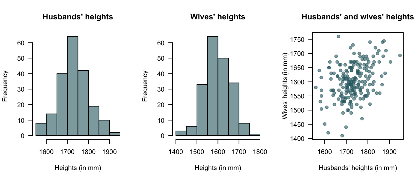
FIGURE 6.9: Plots of the heights data

FIGURE 6.10: Bivariate normal distribution for heights

6.7 Simulation

As with univariate distributions (Sects. 4.9 and 5.7), simulation can be used with bivariate distributions. Random numbers from the bivariate normal distribution (Sect. 6.6.4) are generated using the function dmnorm() from the library mnorm. Random numbers from the multinomial distribution (Sect. 6.6.3) are generated using the function rmultinom(). More commonly, univariate distributions are combined.

Monthly rainfall, for example, is commonly modelled using gamma distributions (for example, Husak, Michaelsen, and Funk (2007)). Simulating rainfall is then used in others models (such as for cropping simulations; for example Ines and Hansen (2006)). As an example, consider a location where the monthly rainfall is well-modelled by a gamma distribution with a shape parameter $\alpha = 1.6$ and a scale parameter of $\beta = 220$ (Fig 6.11, left panel):

library("mnorm") # Need to explicitly load  mnorm  library
#> 
#> Attaching package: 'mnorm'
#> The following objects are masked from 'package:mnormt':
#> 
#>     dmnorm, pmnorm, rmnorm
MRain <- rgamma( 2000,
                 shape = 1.6,
                 scale = 220)

cat("Rainfall exceeding 900mm:",
    sum(MRain > 900) / 2000 * 100, "%\n")
#> Rainfall exceeding 900mm: 4.95 %
# Directly:
round( (1 - pgamma(900, shape = 1.6, scale = 220) ) * 100, 2)
#> [1] 4.95

The percentage of months with rainfall exceeding 1000mm was also computed. However, now suppose that the shape parameter $\alpha$ also varies, with an exponential distribution with mean 2 (Fig 6.11, centre panel):

MRain2 <- rgamma( 1000,
                  shape = rexp(1000, rate = 1/2),
                  scale = 220)

cat("Rainfall exceeding 900mm:",
    sum(MRain2 > 900) / 1000 * 100, "%\n")
#> Rainfall exceeding 900mm: 13.3 %

Using simulation, it is also easy to simulate the impact of the scale parameter $\beta$ varying also, suppose with a normal distribution mean of 200 and variance of 16 (Fig 6.11, right panel):

MRain3 <- rgamma( 1000,
                  shape = rexp(1000, rate = 1/2),
                  scale = rnorm(1000, mean = 200, sd = 4))

cat("Rainfall exceeding 900:",
    sum(MRain3 > 900) / 1000 * 100, "%\n")
#> Rainfall exceeding 900: 11.4 %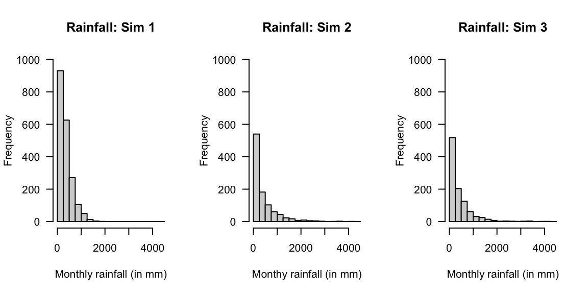

FIGURE 6.11: Three simulations using the gamma distribution

6.8 Exercises

Selected answers appear in Sect. D.6.

Exercise 6.1 The discrete random variables $X$ and $Y$ have the joint pf shown in Table 6.11. Determine:

1. $\Pr(X = 1, Y = 2)$
2. $\Pr(X + Y \le 1)$.
3. $\Pr(X > Y)$.
4. the marginal pf of $X$.
5. the pf of $Y \mid X = 1$.

TABLE 6.11: $X$ and $Y$

	$Y = 0$	$Y = 1$	$Y = 2$
$X = 0$	$1/12$	$1/6$	$1/24$
$X = 1$	$1/4$	$1/4$	$5/24$

Exercise 6.2 The random variable $A$ has mean $13$ and variance $5$. The random variable $B$ has mean $4$ and variance $2$. Assuming $A$ and $B$ are independent, find:

1. $\text{E}(A + B)$.
2. $\text{var}(A + B)$.
3. $\text{E}(2A - 3B)$.
4. $\text{var}(2A - 3B)$.

Exercise 6.3 Repeat Exercise 6.2, but with $\text{cov}(A, B) = 0.2$.

Exercise 6.4 Suppose $X_1, X_2, \dots, X_n$ are independently distributed random variables, each with mean $\mu$ and variance $\sigma^2$. Define the sample mean as $\overline{X} = \left( \sum_{i=1}^n X_i\right)/n$.

1. Prove that $\text{E}(\overline{X}) = \mu$.
2. Find the variance of $\overline{X}$.

Exercise 6.5 The Poisson-gamma distributions (e.g., see Hasan and Dunn (2010)), used for modelling rainfall, can be developed as follows:

• Let $N$ be the number of rainfall events in a month, where $N\sim \text{Pois}(\lambda)$. If no rainfall events are recorded in any month, then the monthly rainfall is $Z = 0$.
• For each rainfall event (that is, when $N > 0$), say $i$ for $i = 1, 2, \dots N$, the amount of rain in event $i$, say $Y_i$, is modelled using a gamma distribution with parameter $\alpha$ and $\beta$.
• The total monthly rainfall is then $Z = \sum_{i = 1}^N Y_i$.

Suppose the monthly rainfall station at a particular station can be modelled using $\lambda = 0.78$, $\alpha = 0.5$ and $\beta = 6$.

1. Use a simulation to produce a one-month rainfall total using this model.
2. Repeat for 1000 simulations (i.e., simulate 1000 months), and plot the distribution.
3. What type of random variable is the monthly rainfall: discrete, continuous, or mixed? Explain.
4. Based on the 1000 simulations, approximately how often does a month have exactly zero rainfall?
5. Based on the 1000 simulations, what is the mean monthly rainfall?
6. Based on the 1000 simulations, what is the mean monthly rainfall in months where rain is recorded?

Exercise 6.6 Suppose $X \sim \text{Pois}(\lambda)$. Show that if $\lambda\sim\text{Gamma}(a, p/(1 - p) )$, then the distribution of $X$ has a negative binomial distribution.

Exercise 6.7 $(X, Y)$ has joint probability function given by $$\Pr(X = x, Y = y) = k |x - y|$$ for $x = 0, 1, 2$ and $y = 1, 2, 3$.

1. Find the value $k$.
2. Construct a table of probabilities for this distribution.
3. Find $\Pr(X \le 1, Y = 3)$.
4. Find $\Pr(X + Y \ge 3)$.

Exercise 6.8 For what value of $k$ is $f(x,y) = kxy$ (for $0 \le x \le 1$; $0 \le y \le 1$, a valid joint pdf?

1. Then, find $\Pr(X \le x_0, Y\le y_0)$.
2. Hence evaluate $\Pr\left(X \le (3/8), Y \le (5/8) \right)$.

Exercise 6.9 $X$, $Y$ and $Z$ are uncorrelated random variables with expected values $\mu_x$, $\mu_y$ and $\mu_z$ and standard deviations $\sigma_x$, $\sigma_y$ and $\sigma_z$. $U$ and $V$ are defined by

$$\begin{align*} U&= X - Z;\\ V&= X - 2Y + Z. \end{align*}$$

1. Find the expected values of $U$ and $V$.
2. Find the variance of $U$ and $V$.
3. Find the covariance between $U$ and $V$.
4. Under what conditions on $\sigma_x$, $\sigma_y$ and $\sigma_z$ are $U$ and $V$ uncorrelated?

Exercise 6.10 Suppose $(X, Y)$ has joint probability function given by $$\Pr(X = x, Y = y) = \frac{|x - y|}{11}$$ for $x = 0, 1, 2$ and $y = 1, 2, 3$.

1. Find $\text{E}(X \mid Y = 2)$.
2. Find $\text{E}(Y \mid X\ge 1)$.

Exercise 6.11 The pdf of $(X, Y)$ is given by $$f_{X, Y}(x, y) = 1 - \alpha(1 - 2x)(1 - 2y),$$ for $0 \le x \le 1$, $0 \le y \le 1$ and $-1 \le \alpha \le 1$.

1. Find the marginal distributions of $X$ and $Y$.
2. Evaluate the correlation coefficient $\rho_{XY}$.
3. For what value of $\alpha$ are $X$ and $Y$ independent?
4. Find $\Pr(X < Y)$.

Exercise 6.12 For the random vector $(X, Y)$, the conditional pdf of $Y$ given $X = x$ is $$f_{Y \mid X = x}(y\mid x) = \frac{2(x + y)}{2x + 1},$$ for $0 < y <1$. The marginal pdf of $X$ is given by $$g_X(x) = x + \frac{1}{2}$$ for $0 <x < 1$.

1. Find $F_Y(y \mid x)$ and hence evaluate $\Pr(Y < 3/4 \mid X = 1/3)$.
2. Find the joint pdf, $f_{X, Y}(x, y)$, of $X$ and $Y$.
3. Find $\Pr(Y < X)$.

Exercise 6.13 The random variables $X_1$, $X_2$, and $X_3$ have y

• $X_1$: mean $\mu_1 = 5$ with standard deviation $\sigma_1 = 2$.
• $X_2$: mean $\mu_2 = 3$ with standard deviation $\sigma_2 = 3$.
• $X_3$: mean $\mu_3 = 6$ with standard deviation $\sigma_3 = 4$.

The correlations are: $\rho_{12} = -\frac{1}{6}$, $\rho_{13} = \frac{1}{6}$ and $\rho_{23} = \frac{1}{2}$.

If the random variables $U$ and $V$ are defined by $U = 2X_1 + X_2 - X_3$ and $V = X_1 - 2X_2 - X_3$, find

1. $\text{E}(U)$.
2. $\text{var}(U)$.
3. $\text{cov}(U, V)$.

Exercise 6.14 Let $X$ and $Y$ be the body mass index (BMI) and percentage body fat for netballers attending the AIS. Assume $X$ and $Y$ have a bivariate normal distribution with $\mu_X = 23$, $\mu_Y = 21$, $\sigma_X = 3$, $\sigma_Y = 6$ and $\rho_{XY} = 0.8$. Find

1. the expected BMI of a netballer who has a percent body fat of 30.
2. the expected percentage body fat of a netballer who has a BMI of 19.

Exercise 6.15 Let $X$ and $Y$ have a bivariate normal distribution with parameters $\mu_x = 1$, $\mu_y = 4$, $\sigma^2_x = 4$, $\sigma^2_y = 9$ and $\rho = 0.6$. Find

1. $\Pr(-1.5 < X < 2.5)$.
2. $\Pr(-1.5 < X < 2.5 \mid Y = 3)$.
3. $\Pr(0 < Y < 8)$.
4. $\Pr(0 < Y < 8 \mid X = 0)$.

Exercise 6.16 In Section 4.6, different forms of the negative binomial distribution were given: one for $Y$, the number of trials until $r$ successes were observed, and for $X$, the number of failures until $r$ successes were observed.

1. Use that $Y = X + r$ to derive the mean and variance of $X$, given that $\text{E}(Y) = r/p$ and $\text{var}(Y) = r(1 - p)/p^2$.
2. Use the mgf for $Y$ to prove the mgf for $X$ is $M_X(t) = \left( \frac{p}{1 - (1 - p)\exp(t)}\right)^r$.

Exercise 6.17 Consider a random process where a fair coin is tossed twice. Let $X$ be the number of heads observed in the two tosses, and $Y$ be the number of heads on the first toss of the coin.

1. Construct the table of the joint probability function for $X$ and $Y$.
2. Determine the marginal probability function for $X$.
3. Determine the conditional distribution of $X$ given one head appeared on the first toss.
4. Determine if the variables $X$ and $Y$ are independent or not, justifying your answer with necessary calculation or argument.

Exercise 6.18 Two fair, six-sided dice are rolled, and the numbers on the top faces. observed. Event $A$ is the maximum of the two numbers, and event $B$ is the minimum of the two numbers.

1. Construct the joint probability function for $A$ and $B$.
2. Determine the marginal distribution for $B$.

Exercise 6.19 Consider $n$ random variables $Z_i$ such that $Z_i \sim \text{Exp}(\beta)$ for every $i = 1, \dots, n$. Show that the distribution of $Z_1 + Z_2 + \cdots + Z_n$ has a gamma distribution $\text{Gam}(n, \beta)$, and determine the parameters of this gamma distribution. (Hint: See Theorem 3.6.)

Exercise 6.20 Daniel S. Wilks (1995b) (p. 101) states that the maximum daily temperatures measured at Ithaca ($I$) and Canandaigua ($C$) in January 1987 are both symmetrical. He also says that the two temperatures could be modelled with a bivariate normal distribution with $\mu_I = 29.87$, $\mu_C = 31.77$, $\sigma_I = 7.71$, $\sigma_C = 7.86$ and $\rho_{IC} = 0.957$. (All measurements are in degrees Fahrenheit.)

1. Explain, in context, what a correlation coefficient of 0.957 means.
2. Determine the marginal distributions of $C$ and of $I$.
3. Find the conditional distribution of $C\mid I$.
4. Plot the pdf of Canandaigua maximum temperature.
5. Plot the conditional pdf of Canandaigua maximum temperature given that the maximum temperature at Ithaca is $25^\circ$F.
6. Comment on the differences between the two pdfs plotted above.
7. Find $\Pr(C < 32 \mid I = 25)$.
8. Find $\Pr(C < 32)$.
9. Comment on the differences between the last two answers.
10. If temperature were measured in degrees Celsius instead of degrees Fahrenheit, how would the value of $\rho_{IC}$ change?

Exercise 6.21 The discrete random variables $X$ and $Y$ have the joint probability distribution shown in the following table:

Value of $x$	$y = 1$	$y = 2$	$y = 3$
$x = 0$	0.20	0.15	0.05
$x = 1$	0.20	0.25	0.00
$x = 3$	0.10	0.05	0.00

1. Determine the marginal distribution of $X$.
2. Calculate $\Pr(X \ne Y)$.
3. Calculate $\Pr(X + Y = 2 \mid X = Y)$.
4. Are $X$ and $Y$ independent? Justify your answer.
5. Calculate the correlation of $X$ and $Y$, $\text{cor}(X,Y)$.

Exercise 6.22 Suppose $X$ and $Y$ have the joint pdf $$f_{X, Y}(x, y) = \frac{2 + x + y}{8} \quad\text{for $-1 < x < 1$ and $-1 < y < 1$}.$$

1. Sketch the distribution using R.
2. Determine the marginal pdf of $X$.
3. Are $X$ and $Y$ independent?
   Give reasons.
4. Determine $\Pr(X > 0, Y > 0)$.
5. Determine $\Pr(X \ge 0, Y \ge 0, X + Y \le 1)$.
6. Determine $\text{E}(XY)$.
7. Determine $\text{var}(Y)$.
8. Determine $\text{cov}(X, Y)$.

Exercise 6.23 Historically, final marks in a certain course are approximately normally distributed with mean of 64 and standard deviation 8. Out of fifteen students completing the course, what is the probability that 2 obtain HDs, 3 Distinctions, 4 Credits, 5 Passes and 2 Fails?

Exercise 6.24 Let $X_1, X_2, X_3, \dots, X_n$ denote are independently and identically distributed with pdf $$f_X(x) = 4x^3\quad \text{for $0 < x < 1$}.$$

1. Write down an expression for the joint pdf of distribution of $X_1, X_2, X_3, \dots, X_n$.
2. Determine the probability that the first observation $X_1$ is less than 0.5.
3. Determine the probability that all observations are less than 0.5.
4. Use the result above to deduce then the probability that the largest observation is less than 0.5.

Exercise 6.25 Let $X$ and $Y$ have a bivariate normal distribution with $\text{E}(X) = 5$, $\text{E}(Y) = -2$, $\text{var}(X) = 4$, $\text{var}(Y) = 9$, and $\text{cov}(X, Y) = -3$. Determine the joint distribution of $U = 3X + 4Y$ and $V = 5X - 6Y$.

Exercise 6.26 Two fair dice are rolled. Let $X$ and $Y$ denote, respectively, the maximum and minimum of the numbers of spots showing on the two dice.

1. Determine $E(Y\mid X = x)$ for $1\le x\le 6$.
2. Simulate this experiment using R. Compare the simulated results with the theoretical results found above.

Exercise 6.27 Let $X$ be a random variable for which $\text{E}(X) = \mu$ and $\text{var}(X) = \sigma^2$, and let $c$ be an arbitrary constant.

1. Show that $$\text{E}[(X - c)^2] = (\mu - c)^2 + \sigma^2.$$
2. What does the result above tell us about the possible size of $\text{E}[(X - c)^2]$?

Exercise 6.28 In Sect. 6.7, simulation was used for monthly rainfall. Daily rainfall, however, is more difficult to model as some days have exactly zero rainfall, and on some days a continuous amount of rainfalls; i.e., daily monthly is a mixed random variable (Sect. 2.2.3).

One way to model daily rainfall is to use a two-step process (Chandler and Wheater 2002). Firstly, model whether a day records rainfall or not (using a binomial distribution): the occurrence model. Then, for days on which rain falls, model the amount of rainfall using a gamma distribution: the amounts model.

1. Use this information to model daily rainfall over one year (365 days), for a location where the probability of a wet day is 0.32, and the amount of rainfall on wet days follows a gamma distribution with $\alpha = 2$ and $\beta = 20$. Produce a histogram of the distribution of annual rainfall after 1000 simulations.
2. Suppose that the probability of rainfall, $p$, depends on the day of the year, such that: $$p = \left\{1 + \cos[ 2\pi\times(\text{day of year})/365]\right\} / 2.2.$$ Plot the change in $p$ over the day of the year.
3. Revise the first model using this value of $p$. Produce a histogram of the distribution of annual rainfall after 1000 simulations.
4. Revise the initial model (where the probability of rain of day 1 is still 0.32), so that the value of $p$ depends on what happened the day before: If day $i$ receives rain, then the probability that the following day receives rain is $p = 0.55$; if day $i$ does not receive rain, then the probability that the following day receives rain is just $p = 0.15$. Produce a histogram of the distribution of annual rainfall after 1000 simulations.

Exercise 6.29 Consider the joint pdf $$f_{X, Y}(x, y) = \begin{cases} c x(y + 1) & \text{where $x + y < 2$ with $x > 0$ and $y > 0$};\\ 0 & \text{elsewhere}. \end{cases}$$

1. Draw the region over which the joint pdf is defined.
2. Compute the value of $c$.
3. Compute $P(Y < 1 \mid X > 1)$.
4. Compute $P(Y < 1 \mid X > 0.25)$.
5. Compute $\Pr(Y < 1)$

Exercise 6.30 Consider the joint pdf $$f_{X, Y}(x, y) = \begin{cases} k ( 1 - x) y & \text{for the region $R$ below};\\ 0 & \text{elsewhere}, \end{cases}$$ where the region $R$ is shown in Fig. 6.12.

1. Determine the value of $k$.
2. Compute $\Pr(X > Y)$.
3. Compute $\Pr(X > 0.5)$.

FIGURE 6.12: The region $R$

Exercise 6.31 A company produces a $500$ g packet of ‘trail mix’ that includes a certain weight of nuts $x$, dried fruit $y$, and seeds $z$. The actually weights of each ingredient vary randomly, depending on seasonality and availability.

1. Explain why there are really just two variables in this problem.
2. Suppose the weight of nuts plus dried fruit must be between $300$ g and $400$ g. Draw the sample space.
3. In addition, suppose the weight of nuts must be at least $100$ g, and the weight of dried fruit must be at least $100$ g. Draw the sample space.
4. Under the above conditions, assume the weights of ingredients used in the trail mix are uniformly distributed. Determine the probability function.

---

Peter K. Dunn, 2024: CC BY-NC-SA 4.0