7 Transformations of random variables

On completion of this module, you should be able to:

• derive the distribution of a transformed variable, given the distribution of the original variable, using the distribution function method, the change of variable method, and the moment-generating function method as appropriate.
• find the joint distribution of two transformed variables in a bivariate situation.

7.1 Introduction

In this chapter, we consider the distribution of a random variable $Y = u(X)$, given a random variable $X$ with known distribution, and a function $u(\cdot)$. Among several available techniques, three are considered:

1. the change of variable method (Sect. 7.2);
2. the distribution function method for continuous random variable only (Sect. 7.3);
3. the moment-generating function method (Sect. 7.4).

An important concept in this context is a one-to-one transformation.

Definition 7.1 (One-to-one transformation) Given random variables $X$ and $Y$ with range spaces $R_X$ and $R_Y$ respectively, the function $u$ is a one-to-one transformation (or mapping) if, for each $y\in R_Y$, there corresponds exactly one $x\in R_X$.

When $Y = u(X)$ is a one-to-one transformation, the inverse function is uniquely defined; that is, $X$ can be written uniquely in terms of $Y$. This is important when considering the distribution of $Y$ when the distribution of $X$ is known.

Example 7.1 The transformation $Y = (X - 1)^2$ is not, in general, a one-to-one transformation. For example, the inverse transformation is $X = 1 \pm \sqrt{Y}$, and two values of $X$ exists for any given value of $Y > 0$ (Fig. 7.1, left panel).

However, if the random variable $X$ is only defined for $X > 2$, then the transformation is a one-to-one function (Fig. 7.1, right panel).

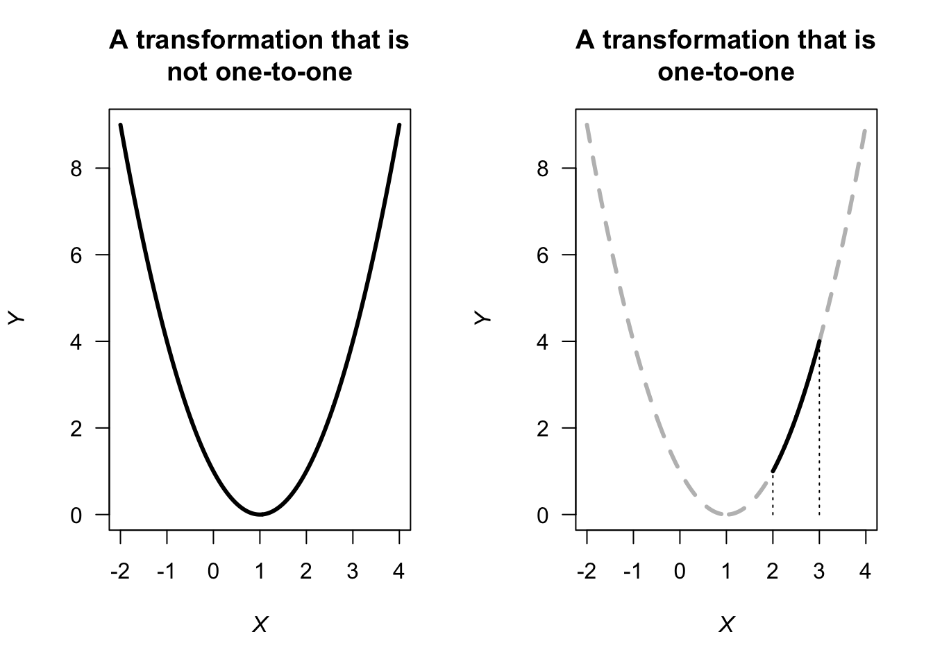
FIGURE 7.1: Two transformations: a non-one-to-one transformation (left panel), and a one-to-one transformation (right panel)

7.2 The change of variable method

The method is relatively straightforward for one-to-one transformations (such as $Y = 1 - X$ or $Y = \exp(X)$). Considerable care needs to be exercised if the transformation is not one-to-one; examples are given below. The discrete and continuous cases are considered separately.

7.2.1 Discrete random variables

7.2.1.1 Univariate case

Let $X$ be a discrete random variable with pf $p_X(x)$. Let $R_X$ denote the set of discrete points for which $p_X(x) > 0$. Let $y = u(x)$ define a one-to-one transformation that maps $R_X$ onto $R_Y$, the set of discrete points for which the transformed variable $Y$ has a non-zero probability. If we solve $y = u(x)$ for $x$ in terms of $y$, say $x = w(y) = u^{-1}(y)$, then for each $y \in R_Y$, we have $x = w(y)\in R_X$.

Example 7.2 (Transformation (1:1)) Given $$p_X(x) = \begin{cases} x/15 & \text{for $x = 1, 2, 3, 4, 5$};\\ 0 & \text{elsewhere}. \end{cases}$$ To find the probability function of $Y$ where $Y = 2X + 1$ (i.e., $u(x) = 2x + 1$), first see that $R_X = \{1, 2, 3, 4, 5\}$. Hence $R_Y = \{3, 5, 7, 9, 11\}$ and the mapping $y = 2x + 1 = u(x)$ is one-to-one. Also, $w(y) = u^{-1}(y) = (y - 1)/2$. Hence, $$\Pr(Y = y) = \Pr(2X + 1 = y) = \Pr\left(X = \frac{y - 1}{2}\right) = \left(\frac{y - 1}{2}\right) \times\frac{1}{15} = \frac{y - 1}{30}.$$ So the probability function of $Y$ is $$\Pr(Y = y) = \begin{cases} (y - 1)/30 & \text{for $y = 3, 5, 7, 9, 11$};\\ 0 & \text{elsewhere}. \end{cases}$$ (Note: The probabilities in this pf add to 1.)

The above procedure when $Y = u(X)$ is a one-to-one mapping can be stated generally as

$$\begin{align*} \Pr(Y = y) &= \Pr\big(u(X) = y\big)\\ &= \Pr\big(X = u^{-1} (y)\big)\\ &= p_X\big(u^{-1}(y)\big), \quad\text{for $y\in R_Y$}. \end{align*}$$

Example 7.3 (Transformation (1:1)) Let $X$ have a binomial distribution with pf $$p_X(x) = \begin{cases} \binom{3}{x}0.2^x (0.8)^{3 - x} & \text{for $x = 0, 1, 2, 3$};\\ 0 & \text{otherwise}. \end{cases}$$ To find the pf of $Y = X^2$, first note that $Y = X^2$ is not a one-to-one transformation in general, but is here since $X$ has non-zero probability only for $x = 0, 1, 2, 3$.

The transformation $y = u(x) = x^2$, $R_X = \{ x \mid x = 0, 1, 2, 3 \}$ maps onto $R_Y = \{y \mid y = 0, 1, 4, 9\}$. The inverse function is $x = w(y) = \sqrt{y}$, and hence the pf of $Y$ is $$p_Y(y) = p_X(\sqrt{y}) = \begin{cases} \binom{3}{\sqrt{y}}0.2^{\sqrt{y}} (0.8)^{3 - \sqrt{y}} & \text{for $y = 0, 1, 4, 9$};\\ 0 & \text{otherwise}. \end{cases}$$

Now consider the case where the function $u$ is not 1:1.

Example 7.4 (Transformation not 1:1) Suppose $\Pr(X = x)$ is as in Example 7.2, and define $Y = |X - 3|$. Since $R_Y = \{0, 1, 2\}$ the mapping is not one-to-one: the event $Y = 0$ occurs if $X = 3$, the event $Y = 1$ occurs if $X = 2$ or $X = 4$, and the event $Y = 2$ occurs if $X = 1$ or $X = 5$. Hence, $R_Y \{ 0, 1, 2\}$.

To find the probability distribution of $Y$: $$\begin{align*} \Pr(Y = 0) &= \Pr(X = 3) = 3/15 = \frac{1}{5};\\ \Pr(Y = 1) &= \Pr(X = 2 \text{ or } 4) = \frac{2}{15} + \frac{4}{15} = \frac{2}{5};\\ \Pr(Y = 2) &= \Pr(X = 1 \text{ or } 5) = \frac{1}{15} + \frac{5}{15} = \frac{2}{5}. \end{align*}$$ The probability function of $Y$ is $$p_Y(y) = \begin{cases} 1/5 & \text{for $y = 0$};\\ 2/5 & \text{for $y = 1$};\\ 2/5 & \text{for $y = 2$};\\ 0 & \text{elsewhere}. \end{cases}$$

7.2.1.2 Bivariate case

The bivariate case is similar to the univariate case. We have a joint pf $p_{X_1, X_2}(x_1, x_2)$ of two discrete random variables $X_1$ and $X_2$ defined on the two-dimensional set of points $R^2_X$ for which $p(x_1, x_2) > 0$. There are now two one-to-one transformations: $$y_1 = u_1( x_1, x_2)\qquad\text{and}\qquad y_2 = u_2( x_1, x_2)$$ that map $R^2_X$ onto $R^2_Y$ (the two-dimensional set of points for which $p(y_1, y_2) > 0$). The two inverse functions are $$x_1 = w_1( y_1, y_2)\qquad\text{and}\qquad x_2 = w_2( y_1, y_2).$$ Then the joint pf of the new (transformed) random variables is $$p_{Y_1, Y_2}(y_1, y_2) = \begin{cases} p_{X_1, X_2}\big( w_1(y_1, y_2), w_2(y_1, y_2)\big) & \text{where $(y_1, y_2)\in R^2_Y$};\\ 0 & \text{elsewhere}. \end{cases}$$

Example 7.5 (Transformation (bivariate)) Let the two discrete random variables $X_1$ and $X_2$ have the joint pf shown in Table 7.1. Consider the two one-to-one transformations $$Y_1 = X_1 + X_2 \qquad\text{and}\qquad Y_2 = 2 X_1.$$ The joint pf of $Y_1$ and $Y_2$ can be found by noting where the $(x_1, x_2)$ pairs are mapped to in the $y_1, y_2$ space:

$(x_1, x_2)$	$\mapsto$	$(y_1,y_2)$
$(-1, 0)$	$\mapsto$	$(-1, -2)$
$(-1, 1)$	$\mapsto$	$(0, -2)$
$(-1, 2)$	$\mapsto$	$(1, -2)$
$(1, 0)$	$\mapsto$	$(1, 2)$
$(1, 1)$	$\mapsto$	$(2, 2)$
$(1, 2)$	$\mapsto$	$(3, 2)$

The joint pf can then be constructed as shown in Table 7.2.

TABLE 7.1: A bivariate probability function

	$x_2 = 0$	$x_2 = 1$	$x_2 = 2$
$x_1 = -1$	$0.3$	$0.1$	$0.1$
$x_1 = +1$	$0.2$	$0.2$	$0.1$

TABLE 7.2: The joint probability function for $Y_1$ and $Y_2$

	$y_1 = -1$	$y_1 = 0$	$y_1 = 1$	$y_1 = 2$	$y_1 = 3$
$y_2 = -2$	$0.3$	$0.1$	$0.1$	$0.0$	$0.0$
$y_2 = +2$	$0.0$	$0.0$	$0.2$	$0.2$	$0.1$

Sometimes, a joint pf of two random variables is given, but only one new random variable is required. In this case, a second (dummy) transformation is used, usually a very simple tranasformation.

Example 7.6 (Transformation (bivariate)) Let $X_1$ and $X_2$ be two independent random variables with the joint pf $$p_{X_1, X_2}(x_1, x_2) = \frac{\mu_1^{x_1} \mu_x^{x_2} \exp( -\mu_1 - \mu_2 )}{x_1!\, x_2!} \quad\text{for $x_1$ and $x_2 = 0, 1, 2, \dots$}$$ This is the joint pf of two independent Poisson random variables. Suppose we wish to find the pf of $Y_1 = X_1 + X_2$.

Consider the two one-to-one transformations, where $Y_2 = X_2$ is just a dummy transformation: $$\begin{align} y_1 &= x_1 + x_2 = u_1(x_1, x_2)\\ y_2 &= x_2\phantom{{} + x_2} = u_2(x_1, x_2) \end{align}$$ which map the points in $R^2_X$ onto $$R^2_Y = \left\{ (y_1, y_2)\mid y_1 = 0, 1, 2, \dots; y_2 = 0, 1, 2, \dots, y_1\right\}.$$ $Y_2$ is a dummy transform, and is very simple. Any second transform could be chosen (as it is not of direct interest), and so choose one that is simple. The inverse functions are

$$\begin{align*} x_1 &= y_1 - y_2 = w_1(y_1, y_2)\\ x_2 &= y_2 \phantom{{} - y_2} = w_2(y_2) \end{align*}$$ by rearranging the original transformations. Then the joint pf of $Y_1$ and $Y_2$ is

$$\begin{align*} p_{Y_1, Y_2}(y_1, y_2) &= p_{X_1, X_2}\big( w_1(y_1, y_2), w_2(y_1, y_2)\big) \\ &= \frac{\mu_1^{y_1 - y_2}\mu_2^{y_2} \exp(-\mu_1 - \mu_2)}{(y_1 - y_2)! y_2!}\quad \text{for $(y_1, y_2)\in R^2_Y$}. \end{align*}$$ Recall that we seek the pf of just $Y_1$, so we need to find the marginal pf of $p_{Y_1, Y_2}(y_1, y_2)$. The marginal pf of $Y_1$ is $$p_{Y_1}(y_1) = \sum_{y_2 = 0}^{y_1} p_{Y_1, Y_2}(y_1, y_2) = \sum_{y_2 = 0}^{y_1} \frac{\mu_1^{y_1 - y_2}\mu_2^{y_2} \exp(-\mu_1 - \mu_2)}{(y_1 - y_2)!\, y_2!},$$ which is equivalent to $$p_{Y_1}(y_1) = \begin{cases} \displaystyle{\frac{(\mu_1 + \mu_2)^{y_1}\exp\big[-(\mu_1 + \mu_2)\big]}{y_1!}} & \text{for $y_1 = 0, 1, 2, \dots$}\\ 0 & \text{otherwise}. \end{cases}$$ You should recognise this as the pf of a Poisson random variable (Def. 4.12) with mean $\mu_1 + \mu_2$. Thus $Y_1 \sim \text{Pois}(\lambda = \mu_1 + \mu_2)$.

7.2.2 Continuous random variables

7.2.2.1 Univariate case

Theorem 7.1 (Change of variable (continuous rv)) If $X$ has pdf $f_X(x)$ for $x\in R_X$ and $u$ is a one-to-one function for $x\in R_X$, then the random variable $Y = u(X)$ has pdf $$f_Y(y) = f_X(x) \left|\frac{dx}{dy}\right|$$ where the RHS is expressed as a function of $y$. The term $\left|dx/dy\right|$ is called the Jacobian of the transformation.

Proof. Let the inverse function be $X = w(Y)$ so that $w(y) = u^{-1}(x)$.

Case 1: $y = u(x)$ is a strictly increasing function (Fig. 7.2, left panel). If $a < y < b$ then $w(a) < x < w(b)$ and $\Pr(a < Y < b) = \Pr\big(w(a) < X <w(b)\big)$, so $${\int^b_a f_Y(y)\,dy =\int^{w(b)}_{w(a)}f_X(x)\,dx =\int^b_af\big( w(y)\big)\frac{dx}{dy}\,\,dy}.$$ Therefore, $\displaystyle {f_Y(y) = f_X\big( w(y) \big)\frac{dx}{dy}}$, where $w(y) = u^{-1}(x)$.

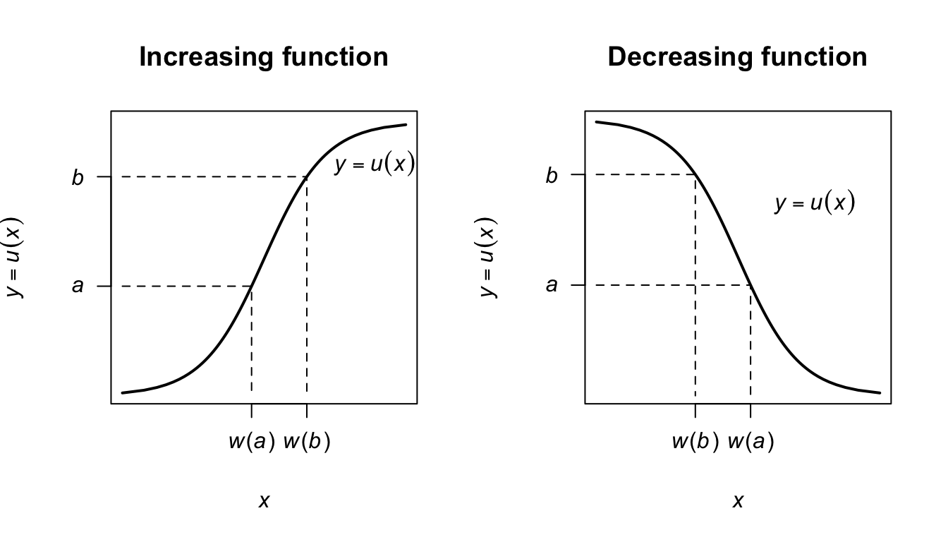
FIGURE 7.2: A strictly increasing transformation function (left panel) and strictly decreasing function (right panel).

Case 2: $y = u(x)$ is a strictly decreasing function of $x$ (Fig. 7.2, right panel). If $a < y < b$ then $w(b) < x < w(a)$ and $\Pr(a < Y < b) = \Pr\big(w(b) < X < w(a)\big)$, so that,

$$\begin{align*} \int^b_a f_Y(y)\,dy & = \int^{w(a)}_{w(b)}f_X(x)\,dx\\ & = \int^a_bf_X(x)\frac{dx}{dy}\,\,dy\\ & = - \int ^b_a f_X(x)\frac{dx}{dy}\,dy. \end{align*}$$ Therefore $f_Y(y) = -f_X\left( w(y) \right)\displaystyle{\frac{dx}{dy}}$. But $dx/dy$ is negative in the case of a decreasing function, so in general $$f_Y(y) = f_X(x)\left|\frac{dx}{dy} \right|.$$

The absolute value of $w'(y) = dx/dy$ is called the Jacobian of the transformation.

Example 7.7 (Transformation) Let the pdf of $X$ be given by $$f_X(x) = \begin{cases} 1 & \text{for $0 < x < 1$};\\ 0 & \text{elsewhere}. \end{cases}$$ Consider the transformation $Y = u(X) = -2\log X$ (where $\log$ refers to logarithms to base $e$, or natural logarithms). The transformation is one-to-one, and the inverse transformation is $$X = \exp( -Y/2) = u^{-1}(Y) = w(Y).$$ The space $R_X = \{x \mid 0 < x < 1\}$ is mapped to $R_y = \{y \mid 0 < y < \infty\}$. Then, $$w'(y) = \frac{d}{dy} \exp(-y/2) = -\frac{1}{2}\exp(-y/2),$$ and so the Jacobian of the transformation $|w'(y)| = \exp(-y/2)/2$. The pdf of $Y = -2\log X$ is $$\begin{align*} f_Y(y) &= f_X\big(w(y)\big) |w'(y)| \\ &= f_X\big(\exp(-y/2)\big) \exp(-y/2)/2 \\ &= \frac{1}{2}\exp(-y/2)\quad\text{for $y > 0$}. \end{align*}$$ That is, $Y$ has an exponential distribution with $\beta = 2$: $Y \sim \text{Exp}(2)$ (Def. 5.8).

Example 7.8 (Square root transformation) Consider the random variable $X$ with pdf $f_X(x) = e^{-x}$ for $x \geq 0$. To find the pdf of $Y = \sqrt{X}$, first see that $y = \sqrt{x}$ is a strictly increasing function for $x \geq 0$ (Fig. 7.3).

The inverse relation is $x = y^2$, and $dx/dy = |2y| = 2y$ for $x \ge 0$. The pdf of $Y$ is $$f_Y(y) = f_X(x)\left|\frac{dx}{dy}\right|\\ = 2y e^{-y^2}\quad \text{for $y\geq0$}.$$

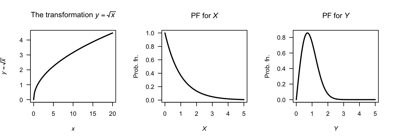
FIGURE 7.3: The square-root transformation (left panel); the pdf of $X$ (centre panel) and the pdf of $Y$ (right panel)

Example 7.9 (Tan transformation) Let random variable $X$ be uniformly distributed on $[-\pi/2, \pi/2]$. Find the distribution of $Y = \tan X$ (Fig. 7.4).

For the mapping $y = \tan x$, we see that $R_Y = \{ y\mid -\infty <y<\infty\}$. The mapping is one-to-one, and so $x = \tan^{-1}y$, and $dx/dy = 1/(1 + y^2)$. Hence $$f_Y(y) = f_X(x)\left|\frac{dx}{dy}\right| = \frac{1}{\pi(1 + y^2)}.$$ This is the Cauchy distribution.

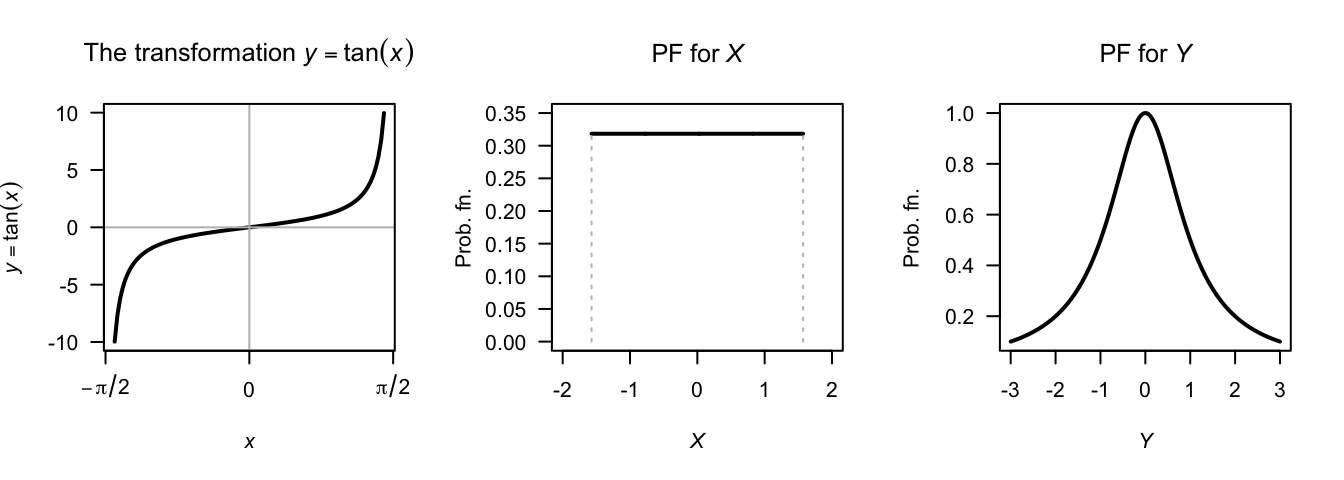
FIGURE 7.4: The tan transformation (left panel); the pdf of $X$ (centre panel) and the pdf of $Y$ (right panel)

A case where the function $u$ is not one-to-one is considered by an example, using a modification of Theorem 7.1.

Example 7.10 (Transformation (not 1:1)) Given a random variable $Z$ which follows a $N(0, 1)$ distribution, find the probability distribution of $Y = \frac{1}{2} Z^2$.

The relationship $y = u(z) = \frac{1}{2}z^2$ is not strictly increasing or decreasing in $(-\infty, \infty )$ so Theorem 7.1 cannot be applied directly. Instead, subdivide the range of $z$ and $y$ so that in each portion the relationship is monotonic. Then: $$f_Z(z) = \frac{1}{\sqrt{2\pi}}\,e^{-\frac{1}{2} z^2}\quad\text{for $-\infty < z < \infty$}.$$ The inverse relation, $z = u^{-1}(y)$ is $z = \pm \sqrt{2y}$. For a given value of $y$, two values of $z$ are possible. In the range $-\infty < z < 0$, $y$ and $z$ are monotonically related. Similarly, for $0 < z <\infty$, $y$ and $z$ are monotonically related. Thus (see Fig. 7.5), $$\Pr(a < Y <b) = \Pr(-\sqrt{2b} < Z < -\sqrt{2a}\,) + \Pr(\sqrt{2a} < Z < \sqrt{2b}\,).$$ The two terms on the right are equal because the distribution of $Z$ is symmetrical about $0$. Thus $\Pr(a < Y < b) = 2\Pr(\sqrt{2a} < Z < \sqrt{2b}\,)$, and $$\begin{align*} f_Y(y) &= 2f_Z(z)\left| \frac{dz}{dy}\right|\\ &= 2\frac{1}{\sqrt{2\pi}}e^{-y}\frac{1}{\sqrt{2y}}; \end{align*}$$ that is, $$f_Y(y) = e^{-y}y^{-\frac{1}{2}} / \sqrt{\pi}\quad\text{for $0 < y < \infty$}.$$ This pdf is a gamma distribution with parameters $\alpha = 1/2$ and $\beta = 1$. It follows that if $X\sim N(\mu,\sigma^2)$, then the pdf of $Y = \frac{1}{2} (X - \mu )^2 / \sigma^2$ is also $\text{Gamma}(\alpha = 1/2,\beta = 1)$ since then $(X - \mu)/\sigma$ is distributed as $N(0, 1)$.

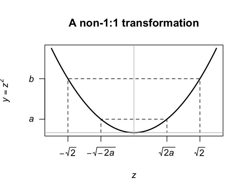
FIGURE 7.5: A transformation not 1:1

Note that the probability can only be doubled as in Example 7.10 if both $Y = u(Z)$ and the pdf of $Z$ are symmetrical about the same point.

7.3 The distribution function method

This method only works for continuous random variables.

There are two basic steps:

1. Find the distribution function of the transformed variable.
2. Differentiate to find the probability density function.

The procedure is best demonstrated using an example.

Example 7.11 (Distribution function method) Consider the random variable $X$ with pdf $$f_X(x) = \begin{cases} x/4 & \text{for $1 < x < 3$};\\ 0 & \text{elsewhere}. \end{cases}$$ To find the pdf of the random variable $Y$ where $Y = X^2$, first see that $1 < y < 9$ and the transfornation is monotonoic over this region. The distribution function for $Y$ is $$\begin{align*} F_Y(y) &= \Pr(Y\le y) \qquad\text{(by definition)}\\ &= \Pr(X^2 \le y) \qquad\text{(since $Y = X^2$)}\\ &= \Pr(X\le \sqrt{y}\,). \end{align*}$$ This last step is not trivial, but is critical. Sometimes, more care is needed (as in the next example). In this case, there is a one-to-one relationship between $X$ and $Y$ over the region of which $X$ is defined (i.e., has a positive probability); see Fig. 7.6.

Then continue as follows:

$$\begin{align*} F_Y(y) =\Pr( X\le \sqrt{y}\,) &= F_X\big(\sqrt{y}\,\big) \qquad\text{(definition of $F_X(x)$)} \\ &= \int_1^{\sqrt{y}} (x/4) \,dx = (y - 1)/8 \end{align*}$$ for $1 < y < 9$, and is zero elsewhere. This is the distribution function of $Y$; to find the pdf: $$f_Y(y) = \frac{d}{dy} (y - 1)/8 = \begin{cases} 1/8 & \text{for $1 < y < 9$};\\ 0 & \text{elsewhere}. \end{cases}$$ Note the range for which $Y$ is defined; since $1 < x < 3$, then $1 < y < 9$.

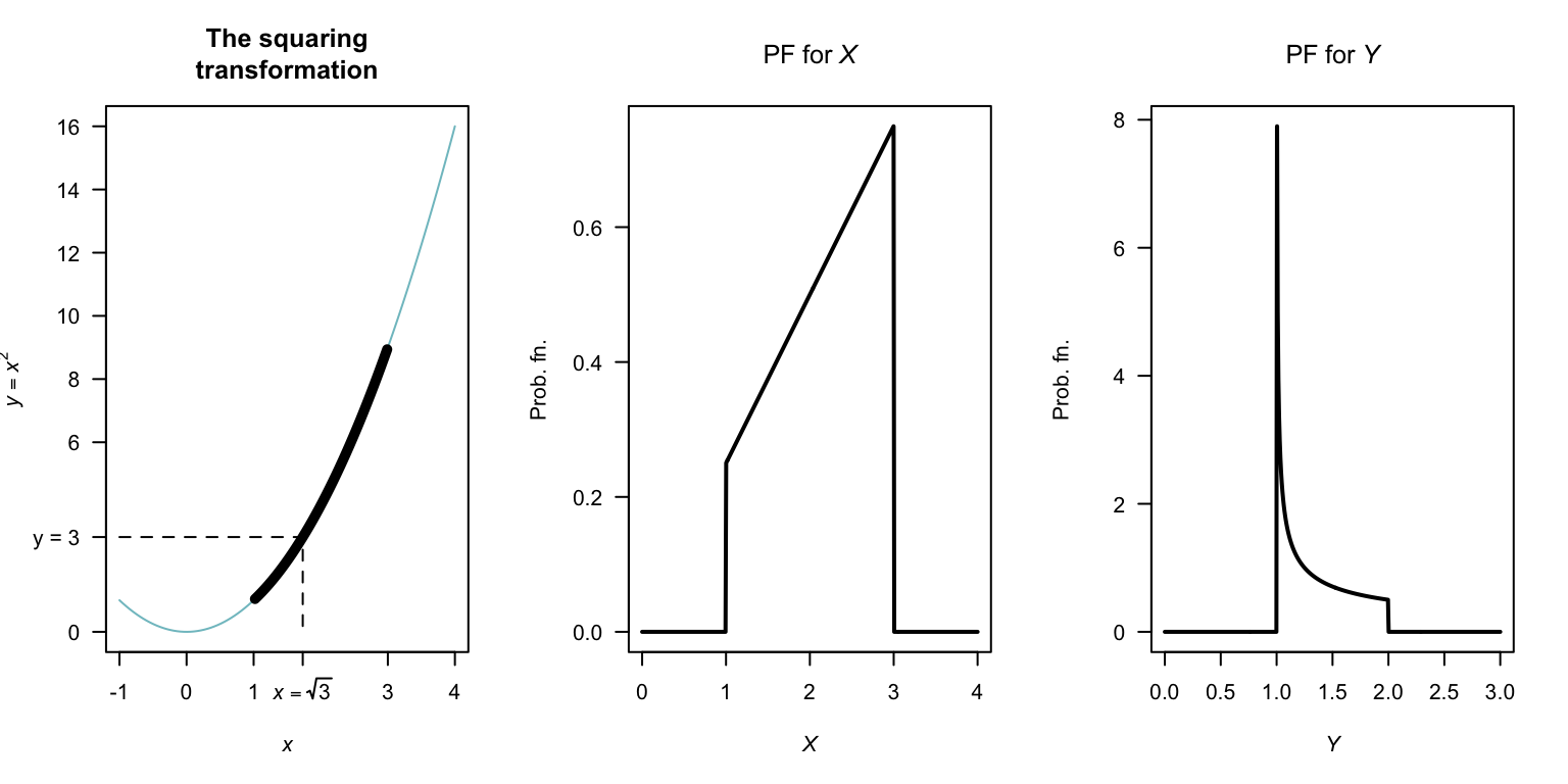
FIGURE 7.6: The transformation $Y = X^2$ when $X$ is defined from $1$ to $3$. The thicker line corresponds to the region where the transformation applies. Note that if $Y < y$, then $2 - \sqrt{y - 1} < X < 2 + \sqrt{y - 1}$.

Example 7.12 (Transformation) Consider the same random variable $X$ as in the previous example, but the transformation $Y = (X - 2)^2 + 1$ (Fig. 7.7).

In this case, the transformation is not a one-to-one transform. Proceed as before to find the distribution function of $Y$:

$$\begin{align*} F_Y(y) &= \Pr(Y\le y) \qquad\text{(by definition)}\\ &= \Pr\big( (X - 2)^2 + 1 \le y\big) \end{align*}$$ since $Y = (X - 2)^2 + 1$. From Fig. 7.7, whenever $(X - 2)^2 + 1 < y$ for some value $y$, then $X$ must be in the range $2 - \sqrt{y - 1}$ to $2 + \sqrt{y - 1}$. So:

$$\begin{align*} F_Y(y) &= \Pr\big( (X - 2)^2 + 1 \le y\big) \\ &= \Pr\left( 2 - \sqrt{y - 1} < X < 2 + \sqrt{y - 1} \right)\\ &= \int_{2-\sqrt{y - 1}}^{2 + \sqrt{y - 1}} x/4\,dx \\ &= \left.\frac{1}{8} x^2\right|_{2 - \sqrt{y - 1}}^{2 + \sqrt{y - 1}} \\ &= \frac{1}{8} \left[ \left(2 + \sqrt{y - 1}\right)^2 - \left(2 - \sqrt{y - 1}\right)^2\right] \\ &= \sqrt{y - 1}. \end{align*}$$ Again, this is the distribution function; so differentiating: $$f_Y(y) = \begin{cases} \frac{1}{2\sqrt{y - 1}} & \text{for $1 < y < 2$};\\ 0 & \text{elsewhere}. \end{cases}$$

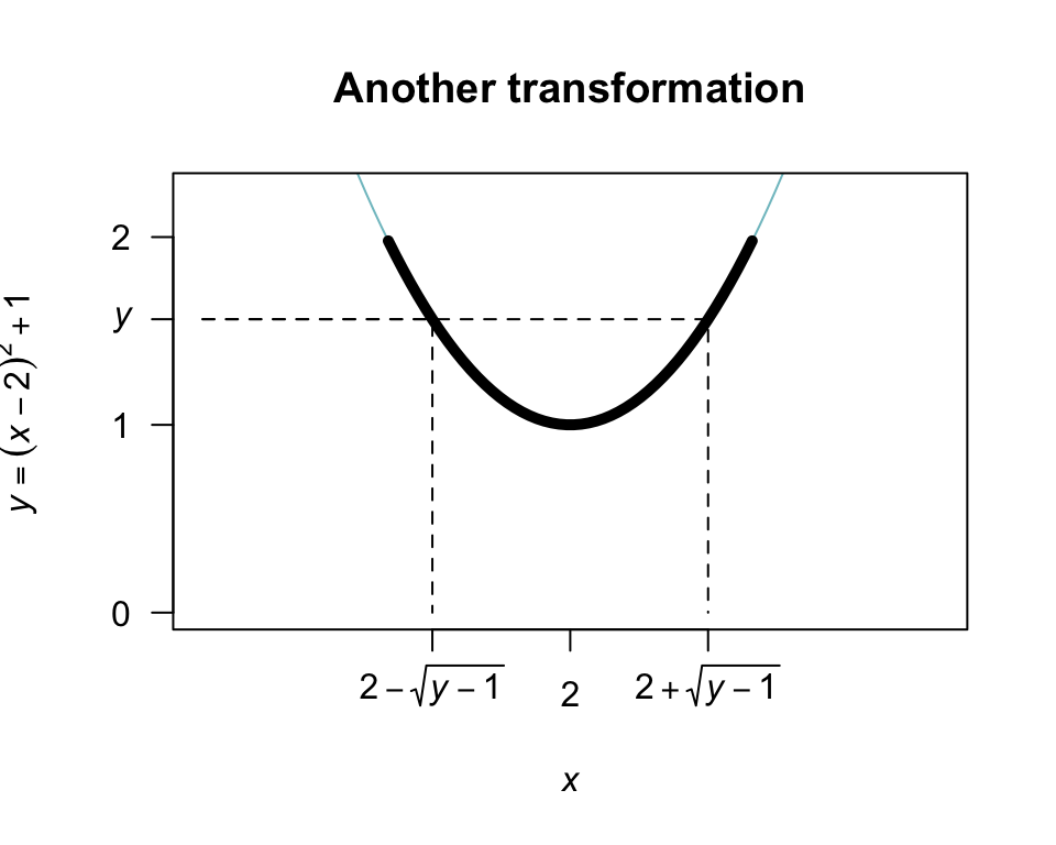
FIGURE 7.7: The transformation $Y = (X - 2)^2 + 1$ when $X$ is defined from $1$ to $3$. The thicker line corresponds to the region where the transformation applies. Note that if $Y < y$, then $2 - \sqrt{y - 1} < X < 2 + \sqrt{y - 1}$.

Example 7.13 (Transformation) Example 7.10 is repeated here using the distribution function method. Given $Z$ is distributed $N(0, 1)$ we seek the probability distribution of $Y = \frac{1}{2} Z^2$. First, $$f_Z(z) = (2\pi )^{-\frac 12}\,e^{-z^2/2}\quad\text{for $z\in (-\infty ,\,\infty )$}.$$ Let $Y$ have pdf $f_Y(y)$ and df $F_Y(y)$. Then $$\begin{align*} F_Y(y) = \Pr(Y\leq y) &= \Pr\left(\frac{1}{2}Z^2\leq y\right)\\ &= \Pr(Z^2\leq 2y)\\ & = \Pr(-\sqrt{2y}\leq Z\leq \sqrt{2y}\,)\\ & = F_Z(\sqrt{2y}\,) - F_Z(-\sqrt{2y}\,) \end{align*}$$ where $F_Z$ is the df of $Z$. Hence

$$\begin{align*} f_Y(y) = F_Y'(y) &= F_Z'(\sqrt{2y}\,)-F_Z'(-\sqrt{2y}\,)\\ &= \frac{\sqrt{2}}{2\sqrt{y}}f_Z(\sqrt{2y}\,) - \frac{\sqrt{2}}{- 2\sqrt{y}}f_Z(-\sqrt{2y}\,)\\[2mm] &= \frac{1}{\sqrt{2y}}[f_Z(\sqrt{2y}\,) + f_Z(-\sqrt{2y}\,)]\\ &= \frac{1}{\sqrt{2y}} \left[ \frac{1}{\sqrt{2\pi}}\,e^{-y}+\frac{1}{\sqrt{2\pi}}\,e^{-y}\right]\\ &= \frac{e^{-y}y^{-\frac{1}{2}}}{\sqrt{\pi}} \end{align*}$$ as before.

Care is needed to ensure the steps are followed logically. Diagrams like Fig. 7.6 and 7.7 are encouraged.

The functions that are produced should be pdfs; check that this is the case.

This method can also be used when there is more than one variable of interest, but we do not cover this.

7.4 The moment-generating function method

The moment-generating function (mgf) method is useful for finding the distribution of a linear combination of $n$ independent random variables. The method essentially involves the computation of the mgf of the transformed variable $Y = u(X_1, X_2, \dots, X_n)$ when the joint distribution of independent $X_1, X_2, \dots, X_n$ is given.

The mgf method relies on this observation: Since the mgf of a random variable (if it exists) completely specifies the distribution of the random variable, then if two random variables have the same mgf they must have identical distributions.

Below, the transformation $Y = X_1 + X_2 + \cdots X_n$ is demonstrated, but the same principles can be applied for other linear combinations also.

Consider $n$ independent random variables $X_1, X_2, \dots, X_n$ with mgfs $M_{X_1}(t)$, $M_{X_2}(t)$, $\dots$, $M_{X_n}(t)$, and consider the transformation $Y = X_1 + X_2 + \cdots X_n$. Since the $X_i$ are independent, $f_{X_1,X_2\dots X_n}(x_1, x_2, \dots, x_n) = f_{X_1}(x_1).f_{X_2}(x_2)\dots f_{X_n}(x_n)$. So, by definition of the mgf,

$$\begin{align*} M_Y(t) &= \text{E}(\exp(tY)) \\ &= \text{E}(\exp[t(X_1 + X_2 + \cdots X_n)]) \\ &= \int\!\!\!\int\!\!\!\cdots\!\!\!\int \exp[t(x_1 + x_2 + \cdots x_n)] f(x_1, x_2, \dots x_n)\,dx_n\dots dx_2\, dx_1 \\ &= \int\!\!\!\int\!\!\!\cdots\!\!\!\int \exp(tx_1) f(x_1) \exp(t{x_2}) f(x_2)\dots \exp(t{x_n})f(x_n) \,dx_n\dots dx_2\, dx_1 \\ &= \int \exp(t x_1) f(x_1)\,dx_1 \int \exp(t{x_2}) f(x_2)\,dx_2 \dots \int \exp(t{x_n})f(x_n)\,dx_n \\ &= M_{X_1}(t) M_{X_2}(t)\dots M_{X_n}(t) \\ &= \prod_{i = 1}^n M_{X_i}(t). \end{align*}$$ ($\prod$ is the symbol for a product of terms, in the same way that $\sum$ is the symbol for a summation of terms.) The above result also holds for discrete variables, where summations replace integrations.

This result follows: If $X_1, X_2, \dots, X_n$ are independent random variables and $Y = X_1 + X_2 + \dots + X_n$, then the mgf of $Y$ is $$M_Y(t) = \prod_{i = 1}^n M_{X_i}(t)$$ where $M_{X_i}(t)$ is the mgf of $X_i$ at $t$ for $i = 1, 2, \dots, n$.

Example 7.14 (Mgf method for transformations) Suppose that $X_i \sim \text{Pois}(\lambda_i)$ for $i = 1, 2, \dots, n$. What is the distribution of $Y = X_1 + X_2 + \dots + X_n$?

Since $X_i$ has a Poisson distribution with parameter $\lambda_i$, the mgf of $X_i$ is $$M_{X_i}(t) = \exp[ \lambda_i(e^t - 1)].$$ The mgf of $Y = X_1 + X_2 + \cdots X_n$ is $$\begin{align*} M_Y(t) &= \prod_{i = 1}^n \exp[ \lambda_i(e^t - 1)] \\ &= \exp[ \lambda_1(e^t - 1)] \exp[ \lambda_2(e^t - 1)] \dots \exp[ \lambda_n(e^t - 1)] \\ &= \exp\left[ (e^t - 1)\sum_{i = 1}^n \lambda_i\right]. \end{align*}$$ Using $\Lambda = \sum_{i = 1}^n \lambda_i$, the mgf of $Y$ is $$M_Y(t) = \exp\left[ (e^t - 1)\Lambda \right],$$ which is the mgf of a Poisson distribution with mean $\Lambda = \sum_{i = 1}^n \lambda_i$. This means that the sum of $n$ independent Poisson distribution is also a Poisson distribution, whose mean is the sum of the individual Poisson means.

7.5 The chi-squared distribution

Examples 7.10 and 7.13 produce the chi-square distribution, which is an important model in statistical theory (Theorem 8.6).

Definition 7.2 (Chi-squared distribution) A continuous random variable $X$ with probability density function

$$\begin{equation} f_X(x) = \frac{x^{(\nu/2) - 1}e^{-x/2}}{2^{\nu/2}\Gamma(\nu/2)}\quad\text{for $x > 0$} \end{equation}$$ is said to have a chi-square distribution with parameter $\nu > 0$. The parameter $\nu$ is called the degrees of freedom. We write $X \sim \chi^2(\nu)$.

Some plots of $\chi^2$-distributions are shown in Fig. 7.8.

The chi-squared is a special case of the gamma distribution with $\alpha = \nu/2$ and $\beta = 2$. This means that properties of the chi-squared distribution can be obtained from those for the gamma distribution.

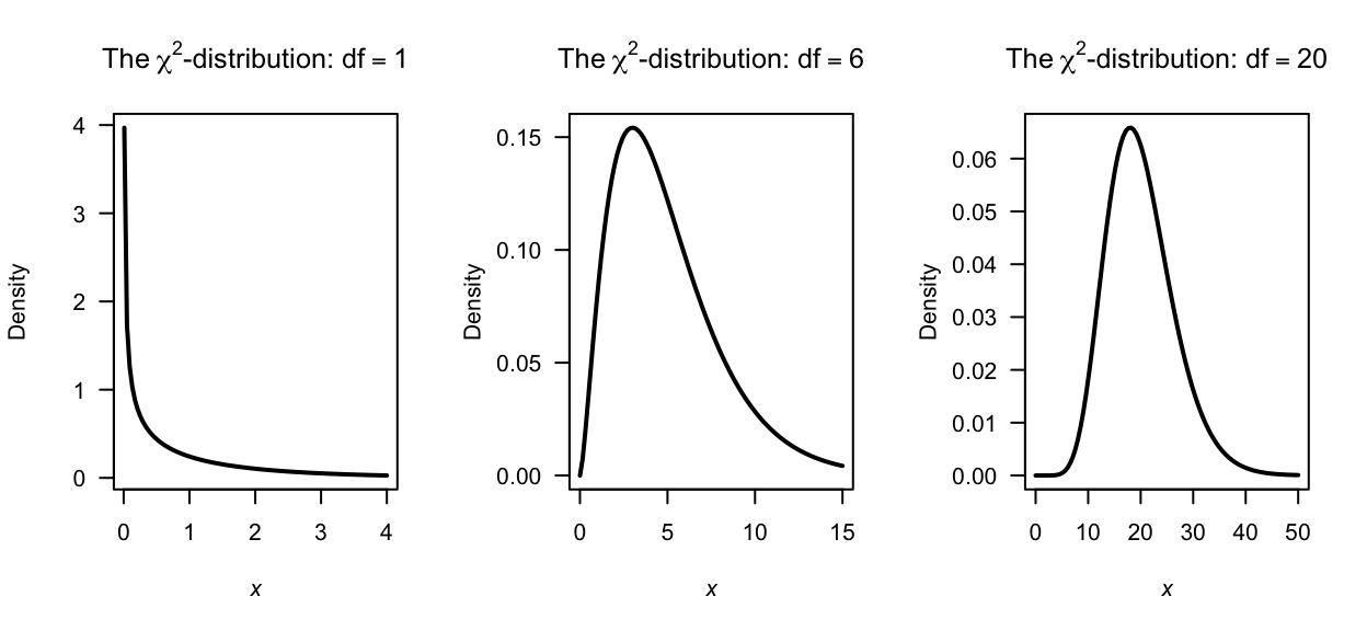
FIGURE 7.8: Some $\chi^2$-distributions

The basic properties of the chi-square follow directly from those of the gamma distribution.

Theorem 7.2 (Properties of chi-squared distribution) If $X\sim\chi^2(\nu)$ then

• $\text{E}(X) = \nu$.
• $\text{var}(X) = 2\nu$.
• $M_X(t) = (1 - 2t)^{-\nu/2}$.

Proof. See Theorem 5.7.

The importance of the chi-square distribution is hinted at in Examples 7.10 and 7.13, which essentially prove the following theorem.

Theorem 7.3 (Chi-square distribution with 1 df) If $Z\sim N(0, 1)$ then $Z^2$ has a chi-square distribution with one degree of freedom.

Proof. Exercise; see Example 7.10.

A useful property of the chi-square distribution is that the sum of independent random variables, each with a chi-square distribution, also has a chi-square distribution. This property is given in the following theorem, which will be used later.

Theorem 7.4 (Chi-squared distribution) If $Z_1, Z_2,\dots, Z_n$ are independently and identically distributed (iid) as $N(0, 1)$, then the sum of squares $S = \sum_i Z_i^2$ has a $\chi^2(n)$ distribution.

Proof. Since $S$ is a linear combination of known distributions, the mgf method is appropriate. Since $Z_i \sim \chi^2(1)$, from Theorem 7.2 $$M_{Z_i}(t) = (1 - 2t)^{-1/2}.$$ From Theorem 3.6 then, $S = \sum_{i = 1}^n Z_i^2$ has mgf $$\begin{align*} M_{S}(t) &= \prod_{i = 1}^n (1 - 2t)^{-1/2}\\ &= \left[(1 - 2t)^{-1/2}\right]^n = (1 - 2t)^{-n/2}, \end{align*}$$ which is the mgf of $\chi^2(n)$.

Chi-square probabilities cannot in general be calculated without computers or tables.

The four R functions for working with the chi-squared distribution have the form [dpqr]chisq(df), where df${} = \nu$ refers to the degrees of freedom (see Appendix B).

Example 7.15 (Chi-squared distributions) The variable $X$ has a chi-square distribution with 12 df. Determine the value of $X$ below which lies 90% of the distribution.

We seek a value $c$ such that $\Pr(X < c) = F_X(c) = 0.90$ where $X\sim\chi^2(12)$. In R:

qchisq(0.9, df = 12)
#> [1] 18.54935

That is, about 90% of the distribution lies below 18.549.

7.6 Exercises

Selected answers appear in Sect. D.7.

Exercise 7.1 Suppose the pdf of $X$ is given by $$f_X(x) = \begin{cases} x/2 & \text{$0 < x < 2$};\\ 0 & \text{otherwise}. \end{cases}$$

1. Find the pdf of $Y = X^3$ using the change of variable method.
2. Find the pdf of $Y = X^3$ using the distribution function method.

Exercise 7.2 The discrete bivariate random vector $(X_1, X_2)$ has the joint pf $$f_{X_1, X_2}(x_1, x_2) = \begin{cases} (2x_1+ x _2)/6 & \text{for $x_1 = 0, 1$ and $x_2 = 0, 1$};\\ 0 & \text{elsewhere}. \end{cases}$$ Consider the transformations

$$\begin{align*} Y_1 &= X_1 + X_2 \\ Y_2 &= \phantom{X_1+{}} X_2 \end{align*}$$

1. Determine the joint pf of $(Y_1, Y_2)$.
2. Deduce the distribution of $Y_1$.

Exercise 7.3 Consider $n$ random variables $X_i$ such that $X_i \sim \text{Gam}(\alpha_i, \beta)$. Determine the distribution of $Y = \sum_{i = 1}^n X_i$ using mgfs.

Exercise 7.4 The random variable $X$ has pdf $$f_X(x) = \frac{1}{\pi(1 + x^2)}$$ for $-\infty < x < \infty$. Find the pdf of $Y$ where $Y = X^2$.

Exercise 7.5 A random variable $X$ has distribution function $$F_X(x) = \begin{cases} 0 & \text{for $x \le -0.5$};\\ \frac{2x + 1}{2} & \text{for $-0.5 < x < 0.5$};\\ 1 & \text{for $x \ge 0.5$}. \end{cases}$$

1. Find, and plot, the pdf of $X$.
2. Find the distribution function, $F_Y(y)$, of the random variable $Y = 4 - X^2$.
3. Hence find, and plot, the pdf of $Y$, $f_Y(y)$.

Exercise 7.6 Suppose a projectile is fired at an angle $\theta$ from the horizontal with velocity $v$. The horizontal distance that the projectile travels, $D$, is $$D = \frac{v^2}{g} \sin 2\theta,$$ where $g$ is the acceleration due to gravity ($g\approx 9.8$ m.s^$-2$).

1. If $\theta$ is uniformly distributed over the range $(0, \pi/4)$, find the probability density function of $D$.
2. Sketch the pdf of $D$ over a suitable range for $v = 12$ and using $g\approx 9.8$$m.s².

Exercise 7.7 Most computers have facilities to generate continuous uniform (pseudo-)random numbers between zero and one, say $X$. When needed, exponential random numbers are obtained from $X$ using the transformation $Y = -\alpha\ln X$.

1. Show that $Y$ has an exponential distribution and determine its parameters.
2. Deduce the mean and variance of $Y$.

Exercise 7.8 Consider a random variable $W$ for which $\Pr(W = 2) = 1/6$, $\Pr(W = -2) = 1/3$ and $\Pr(W = 0) = 1/2$.

1. Plot the probability function of $W$.
2. Find the mean and variance of $W$.
3. Determine the distribution of $V = W^2$.
4. Find the distribution function of $W$.

Exercise 7.9 In a study to model the load on bridges (Lu, Ma, and Liu 2019), the researchers modelled the Gross Vehicle Weight (GVM, in kilonewtons) weight of smaller trucks $S$ using $S\sim N(390, 740$, and the weight of bigger trucks $B$ using $L\sim N(865, 142)$. The total load distribution $L$ was then modelled as $L = 0.24S + 0.76B$.

1. Plot the distribution of $L$.
2. Compute the mean and standard deviation of $L$.

Exercise 7.10 Suppose the random variable $X$ has a normal distribution with mean $\mu$ and variance $\sigma^2$. The random variable $Y = \exp X$ is said to have a log-normal distribution.

1. Determine the df of $Y$ in terms of the function $\Phi(\cdot)$ (see Def. 5.7).
2. Differentiate to find the pdf of $Y$.
3. Plot the log-normal distribution for various parameter values.
4. Determine $\Pr(Y > 2 | Y < 1)$ when $\mu = 2$ and $\sigma^2 = 2$.

(Hint: Use the dlnorm() and plnorm() functions in R, where $\mu = {}$meanlog and $\sigma = {}$sdlog.)

Exercise 7.11 If $X$ is a random variable with probability function $$\Pr(X = x) = \binom{4}{x} (0.2)^x (0.8)^{4 - x} \quad \text{for $x = 0, 1, 2, 3, 4$},$$ find the probability function of the random variable defined by $Y = \sqrt{X}$.

Exercise 7.12 Given the random variable $X$ with probability function $$\Pr(X = x) = \frac{x^2}{30} \quad \text{for $x = 1, 2, 3, 4$},$$ find the probability function of $Y= (X - 3)^2$.

Exercise 7.13 A random variable $X$ has distribution function $$F_X(x) = \begin{cases} 0 & \text{for $x < -0.5$};\\ \frac{2x + 1}{2}, & \text{for $-0.5 < x < 0.5$}; \\ 1 & \text{for $x > 0.5$}. \end{cases}$$

1. Find the distribution function, $F_Y(y)$, of the random variable $Y = 4 - X^2$.
2. Hence find the pdf of $Y$, $f_Y(y)$.

Exercise 7.14 If the random variable $X$ has an exponential distributed with mean 1, show that the distribution of $-\log(X)$ has a Gumbel distribution (Eq. (3.6)) with $\mu = 0$ and $\sigma = 1$.

Exercise 7.15 Let $X$ have a gamma distribution with parameters $\alpha > 2$ and $\beta > 0$.

1. Prove that the mean of $1/X$ is $\beta/(\alpha - 1)$.
2. Prove that the variance of $1/X$ is $\beta^2/[(\alpha - 1)^2(\alpha - 2)]$.

Exercise 7.16 In a study modelling waiting times at a hospital (Khadem et al. 2008), patients are classified into one of three categories:

• Red: Critically ill or injured patients.
• Yellow: Moderately ill or injured patients.
• Green: Minimally injured or uninjured patients.

For ‘Green’ patients, the service time $S$ was modelled as $S = 4.5 + 11V$, where $V \sim \text{Beta}(0.287, 0.926)$.

1. Produce well-labelled plots of the pdf and df of $S$, showing important features.
2. What proportion of patients have a service time exceeding $15$ mins?
3. The quickest $20$% of patients are serviced within what time?

Exercise 7.17 In a study modelling waiting times at a hospital (Khadem et al. 2008), patients are classified into one of three categories:

• Red: Critically ill or injured patients.
• Yellow: Moderately ill or injured patients.
• Green: Minimally injured or uninjured patients.

The time (in minutes) spent in the reception are for ‘Yellow’ patients, say $T$, is modelled as $T = 0.5 + W$, where $W\sim \text{Exp}(16.5)$.

1. Plot the pdf and df of $T$.
2. What proportion of patients waits more than $20$ mins, if they have already been waiting for $10$ mins?
3. How long to the slowest $10$% of patients need to wait?

Exercise 7.18 Suppose the random variable $Z$ has the pdf
$$f_Z(z) = \begin{cases} \frac{1}{3} & \text{for $-1 < z < 2$};\\ 0 & \text{elsewhere}. \end{cases}$$

1. Find the probability density function of $Y$, where $Y = Z^2$, using the distribution function method.
2. Confirm that your final pdf of $Y$ is a valid pdf.
3. Produce a well-labelled plot of the pdf of $Y$. Ensure all important points, etc. are clearly labelled.

---

Peter K. Dunn, 2024: CC BY-NC-SA 4.0