5 Standard continuous distributions

On completion of this module, you should be able to:

• recognise the probability functions and underlying parameters of uniform, exponential, gamma, beta, and normal random variables.
• know the basic properties of the above continuous distributions.
• apply these distributions as appropriate to problem solving.
• approximate the binomial distribution by a normal distribution.

5.1 Introduction

In this chapter, some popular continuous distributions are discussed. Properties such as definitions and applications are considered.

5.2 Continuous uniform distribution

The continuous uniform distribution has a constant pdf over a given range.

Definition 5.1 (Continuous uniform distribution) If a random variable \(X\) with range space \([a, b]\) has the pdf
\[\begin{equation} f_X(x; a, b) = \displaystyle\frac{1}{b - a}\quad\text{for $a\le x\le b$}, \tag{5.1} \end{equation}\] then \(X\) has a continuous uniform distribution. We write \(X\sim U(a, b)\) or \(X\sim\text{Unif}(a, b)\).

This distribution is also called the rectangular distribution. The same notation is used to denote the discrete and continuous uniform distribution; the context should make it clear which is meant. A plot of the pdf for a continuous uniform distribution is shown in Fig. 5.1.

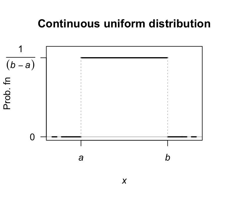
Figure 5.1: The pdf for a continuous uniform distribution \(U(a,b)\).

Definition 5.2 (Continuous uniform distribution: distribution function) For a random variable \(X\) with the continuous uniform distribution given in (5.1), the distribution function is
\[ F_X(x; a, b) = \begin{cases} 0 & \text{for $x < a$};\\ \displaystyle \frac{x - a}{b - a} & \text{ for $a \le x \le b$};\\ 1 & \text{for $x > b$}. \end{cases} \]

The following are the basic properties of the continuous uniform distribution.

Theorem 5.1 (Continuous uniform distribution properties) If \(X\sim\text{Unif}(a,b)\) then

1. \(\text{E}(X) = (a + b)/2\).
2. \(\text{var}(X) = (b - a)^2/12\).
3. \(M_X(t) = \{ \exp(bt) - \exp(at) \} / \{t(b - a)\}\).

Proof. These proofs are left as exercises.

The four R functions for working with the continuous uniform distribution have the form [dpqr]unif(min, max) (see Appendix B).

Example 5.1 (Continuous uniform) If \(X\) is uniformly distributed on \([-2, 2]\), then \(\Pr(|X| > \frac{1}{2})\) can be found. Note that
\[ f_X(x; a = =2, b = 2) = \frac{1}{4} \quad\text{for $-2 < 2$.} \] Then:
\[\begin{align*} \Pr\left(|X| > \frac{1}{2}\right) &= \Pr\left(X > \frac{1}{2}\right) + \Pr\left(X < -\frac{1}{2}\right)\\ &= \int^2_{\frac{1}{2}} f(x)\,dx + \int^{-\frac{1}{2}}_{-2} f(x)\,dx\\ &= \frac{3}{4}. \end{align*}\] The probability could also be computed by finding the area of the appropriate rectangle. Alternatively, in R:

punif(-0.5, -2, 2) + 
  1 - punif(0.5, -2, 2)
#> [1] 0.75

5.3 Normal distribution

5.3.1 Definition and properties

The most well-known continuous distribution is probably the normal distribution (or Gaussian distribution), sometimes called the bell-shaped distribution. The normal distribution has many applications (especially in sampling), and many natural quantities (such as heights and weights of humans) follow normal distributions.

Definition 5.3 (Normal distribution) If a random variable \(X\) has the pdf
\[\begin{equation} f_X(x; \mu, \sigma^2) = \displaystyle \frac{1}{\sigma \sqrt{2\pi}} \exp\left\{ -\frac{1}{2}\left( \frac{x-\mu}{\sigma}\right)^2 \right\} \tag{5.2} \end{equation}\] for \(-\infty<x<\infty\), then \(X\) has a normal distribution. The two parameters are the mean \(\mu\) such that \(-\infty < \mu < \infty\); and the variance \(\sigma^2\) such that \(\sigma^2 > 0\). We write \(X\sim N(\mu, \sigma^2)\).

Some authors—especially in non-theoretical work—use the notation \(X\sim N(\mu,\sigma)\) so it is wise to check each article or book for the notation used. Some examples of normal distribution pdfs are shown in Fig. 5.2.

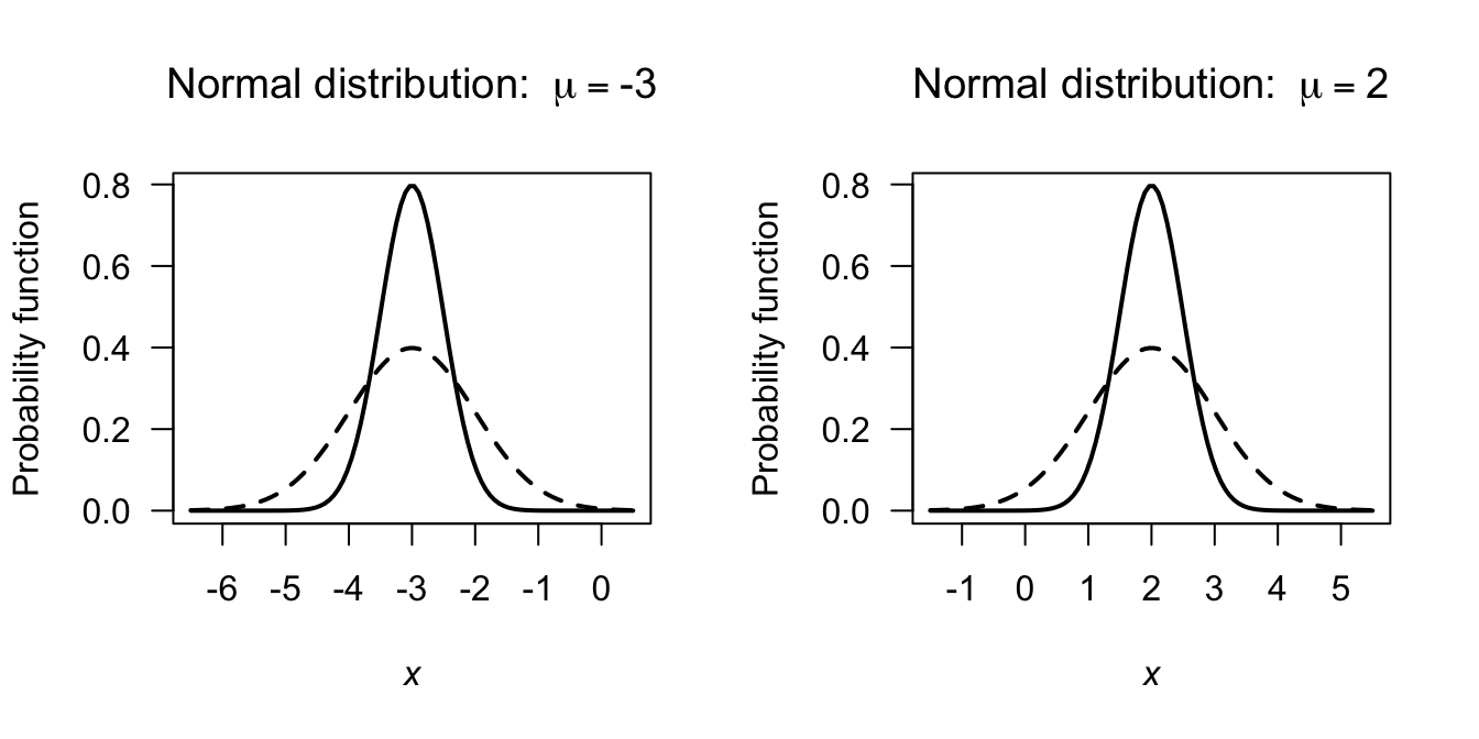
Figure 5.2: Some examples of normal distributions. The solid lines correspond to \(\sigma = 0.5\) and the dashed lines to \(\sigma = 1\). For the left panel, \(\mu = -3\); for the right panel, \(\mu = 2\).

In drawing the graph of the normal pdf, note that

1. \(f_X(x)\) is symmetrical about \(\mu\): \(f_X(\mu - x) = f_X(\mu + x)\).
2. \(f_X(x) \to 0\) asymptotically as \(x\to \pm \infty\).
3. \(f_X'(x) = 0\) when \(x = \mu\), and a maximum occurs there.
4. \(f_X''(x) = 0\) when \(x = \mu \pm \sigma\) (points of inflexion).

The proof that \(\displaystyle \int^\infty_{-\infty} f_X(x)\,dx = 1\) is not obvious so will not be given. The proof relies on first squaring the integral and then changing to polar coordinates.

Definition 5.4 (Normal distribution: distribution function) For a random variable \(X\) with the normal distribution given in (5.2), the distribution function is
\[\begin{align} F_X(x; \mu, \sigma^2) = \frac{1}{\sigma \sqrt{2\pi}} \int_{-\infty}^x \exp\left\{\frac{(t - \mu)^2}{2\sigma^2}\right\}\, dt\\ = \frac{1}{2} \left\{1 + \operatorname{erf} \left( \frac{x - \mu}{\sigma {\sqrt{2}} }\right)\right\} \end{align}\] where \(\operatorname{erf}(\cdot)\) is the error function
\[\begin{equation} \operatorname{erf}(x) = \frac{2}{\sqrt{\pi}} \int _{0}^{x} \exp\left( -t^{2}\right)\,dt, \tag{5.3} \end{equation}\] for \(x \in\mathbb{R}\). The function \(\operatorname{erf}(\cdot)\) appears in numerous places, is commonly tabulated, and available in many computer packages.

The following are the basic properties of the normal distribution.

Theorem 5.2 (Normal distribution properties) If \(X\sim N(\mu,\sigma^2)\) then

1. \(\text{E}(X) = \mu\).
2. \(\text{var}(X) = \sigma^2\).
3. \(M_X(t) = \displaystyle \exp\left(\mu t + \frac{t^2\sigma^2}{2}\right)\).

Proof. The proof is delayed until after the Theorem 5.3.

The four R functions for working with the normal distribution have the form [dpqr]norm(mean, sd) (see Appendix B). Note that the normal distribution is specified by giving the standard deviation and not the variance.

The error function \(\operatorname{erf}(\cdot)\) is not available directly in R, but can be evaluated using
\[ \operatorname{erf}(\cdot) = 2\times \texttt{pnorm}(x\sqrt{2}) - 1. \]

5.3.2 The standard normal distribution

A special case of the normal distribution is the standard normal distribution, when the normal distribution has mean zero and variance one.

Definition 5.5 (Standardard normal distribution) The pdf for a random variable \(Z\) with a standard normal distribution is
\[ f_Z(z) = \displaystyle \frac{1}{\sqrt{2\pi}} \exp\left\{ -\frac{z^2}{2}\right\} \tag{5.4} \] where \(-\infty < z < \infty\). We write \(Z\sim N(0, 1)\).

Since \(f_Z(z)\) is a pdf, then
\[\begin{equation} \frac 1{\sqrt{2\pi}}\int^\infty_{-\infty} \exp\left\{-\frac{1}{2} z^2\right\}\,dz = 1, \tag{5.5} \end{equation}\] a result which proves useful in many contexts (as in the proof of the second statement in 4.7, and in the proof below).

Definition 5.6 (Standard normal distribution: distribution function) For a random variable \(X\) with the standard normal distribution given in (5.4), the distribution function is
\[\begin{align} F_X(x) &= \frac{1}{2} \left\{1 + \operatorname{erf} \left( \frac {x}{\sqrt{2}} \right)\right\}\nonumber\\ &= \int_{-\infty}^z \frac{1}{\sqrt{2\pi}} \exp\left\{ -\frac{t^2}{2}\right\}\, dt \\ &= \Phi(z) \tag{5.6} \end{align}\] where \(\operatorname{erf}(\cdot)\) is the error function (5.3).

Definition 5.7 (Notation) The distribution function for the standard normal distribution is used so often that is has its own notation: \(\Phi(\cdot)\). The distribution function of a normal distribution with mean \(\mu\) and standard deviation \(\sigma\) is then denoted \(\Phi\big( (x - \mu)/\sigma\big)\).

Analogously, the pdf of the standard normal distribution is sometimes denoted by \(\phi(\cdot)\), and hence the PDF of a normal distribution with mean \(\mu\) and standard deviation \(\sigma\) is then denoted \(\phi\big( (x - \mu)/\sigma\big)\).

Note: \(\displaystyle\frac{d}{dx} \Phi(x) = \phi(x)\).

The following are the basic properties of the standard normal distribution.

Theorem 5.3 (Standard normal distribution properties) If \(Z\sim N(0, 1)\) then

1. \(\text{E}(Z) = 0\).
2. \(\text{var}(Z) = 1\).
3. \(M_Z(t) = \displaystyle \exp\left(\frac{t^2}{2}\right)\).

Proof. Part 3 could be proven first, and used to prove Parts 1 and 2. However, proving Parts 1 and 2 directly is constructive. For the expected value:
\[\begin{align*} \text{E}(Z) &= \frac {1}{\sqrt{2\pi}} \int^\infty_{-\infty} z \exp\left\{-\frac{1}{2}z^2 \right\}\,dz\\ &= \int^\infty_{-\infty} -\frac{d}{dz} \left(\exp\left\{-\frac{1}{2}z^2\right\} \right)\, dz\\ &= \left[ -\exp\left\{-\frac{1}{2}z^2\right\}\right]^\infty_{-\infty} = 0, \end{align*}\] since the integrand is symmetric about \(0\).

For the variance, first see that \(\text{var}(Z) = \text{E}(Z^2) - \text{E}(Z)^2 = \text{E}(Z^2)\) since \(\text{E}(Z) = 0\). So:
\[ \text{var}(X) = \text{E}(Z^2) = \frac {1}{\sqrt{2\pi}}\int^\infty_{-\infty}z^2e^{-\frac{1}{2}z^2}\,dz. \] To integrate by parts (i.e., \(\int u\,dv = uv - \int v\, du\)), set \(u = z\) (so that \(du = 1\)) and set
\[ dv = ze^{-\frac{1}{2}z^2} \quad\text{so that}\quad v = -e^{-\frac{1}{2}z^2}. \] Hence,
\[\begin{align*} \text{var}(X) &= \frac {1}{\sqrt{2\pi}} \left\{ -z \exp\left\{-\frac{1}{2}z^2\right\} - \int^\infty_{-\infty}-\exp\left\{-\frac{1}{2}z^2\right\}\, dz \right\}\\ &= \frac {1}{\sqrt{2\pi}}\left(\left. -z\,\exp\left\{-\frac{1}{2} z^2\right\}\right|^\infty_{-\infty}\right) + \frac{1}{\sqrt{2\pi}}\int^\infty_{-\infty} \exp\left\{-\frac{1}{2}z^2\right\}\,dz = 1 \end{align*}\] since the first term is zero, and the second term uses (5.5).

For the mgf:
\[ M_Z(t) = \text{E}(\exp\left\{tZ\right\}) = \int^\infty_{-\infty} \exp\left\{tz\right\} \frac{1}{\sqrt{2\pi}} \exp\left\{-\frac{1}{2}z^2\right\}\,dz. \] Collecting together the terms in the exponent and completing the square,
\[\begin{equation*} -\frac{1}{2}[z^2 -2tz] = -\frac{1}{2}(z - t)^2+\frac{1}{2} t^2. \end{equation*}\] Taking the constants outside the integral:
\[ M_Z(t) = \exp\left\{\frac{1}{2}t^2\right\}\int^\infty_{-\infty} \frac{1}{\sqrt{2\pi}} \exp\left\{-\frac{1}{2}[z - t]^2\right\}\,dz. \] The integral here is 1, since it is the area under an \(N(t, 1)\) pdf. Hence
\[ M_Z(t) = \exp\left\{\frac{1}{2} t^2\right\}. \]

This distribution is important in practice since any normal distribution can be rescaled into a standard normal distribution using
\[\begin{equation} Z = \frac{X - \mu}{\sigma}. \tag{5.7} \end{equation}\] Since \(Z = (X - \mu)/\sigma\), then \(X = \mu + \sigma Z\), and so
\[ \text{E}(X) = \text{E}(\mu + \sigma Z) = \mu + \sigma \text{E}(Z) = \mu \] because \(\text{E}(Z) = 0\). Also
\[ \text{var}(X) = \text{var}(\mu +\sigma Z) = \sigma^2\text{var}(Z) = \sigma^2 \] because \(\text{var}(Z) = 1\). Finally
\[ M_X(t) = \text{E}(e^{tX}) = \text{E}\big(\exp\{t(\mu + \sigma Z)\}\big) = \exp(\mu t)\text{E}\big(\exp(t\sigma Z)\big). \] However, \(\text{E}\big(\exp(t\sigma Z)\big) = M_Z(t\sigma) = \exp\left\{\frac{1}{2}(\sigma t)^2\right\}\) so
\[ M_Z(t) = \displaystyle \exp\left(\frac{t^2}{2}\right). \]

The four R functions for working with the normal distribution have the form [dpqr]norm(mean, sd) (see Appendix B). By default, mean = 0 and sd = 1, corresponding to the standard normal distribution. Note that the normal distribution is specified by giving the standard deviation and not the variance.

5.3.3 Determining normal probabilities

The probability \(\Pr(a < X \le b)\) where \(X\sim N(\mu, \sigma^2)\) can be written
\[ \Pr(a < X \le b) = F_X(b) - F_X(a). \] where \(F_X(x)\) is the distribution function in Def. 5.6. The integral in the distribution function cannot be written in terms of standard functions and in general must be evaluated for a particular \(x\) numerically (e.g., using Simpson’s rule or similar). However, all statistical packages have built-in procedures to evaluate \(F_X(x)\) for any \(z\) (such as pnorm() in R).

Also, since any normal distribution can be transformed into a standard normal distribution, we can write
\[ z_1 = (a - \mu)/\sigma \quad\text{and}\quad z_2 = (b - \mu)/\sigma \] and hence the probability is
\[ \Pr( z_1 < Z \le z_2) = \Phi(z_2) - \Phi(z_1), \] where \(\Phi(z)\) is the distribution function for the standard normal distribution (5.3).

The process of converting a value \(x\) into \(z\) using \(z = (x - \mu)/\sigma\) is called standardising. Tables of \(\Phi(z)\) (or sometimes \(1 - \Phi(z)\)) are commonly available. These tables can be used to compute any probabilities associated with the normal distributions (see the examples below). Of course, R can be used too.

In addition, the tables are often used in the reverse sense, where the probability of an event is given and the value of the random variable is sought. In these case, the tables are used ‘backwards’; the appropriate area is found in the body of the table and the corresponding \(z\)-value found in the table margins. In R, the function qnorm() is used. This \(z\)-value is then converted to a value of the original random variable using
\[\begin{equation} x = \mu + z\sigma. \tag{5.8} \end{equation}\] This process is sometimes referred to as unstandardising.

The following examples illustrate the use of R. Drawing rough graphs showing the relevant areas is encouraged.

Example 5.2 (Walking speeds) A study of stadium evacuations used a simulation to compare scenarios (H. Xie, Weerasekara, and Issa 2017). The walking speed of people was modelled using a \(N(1.15, 0.2^2)\) distribution; that is, \(\mu = 1.15\) m/s with a standard deviation of 0.2m/s. The situation can be shown in Fig. 5.3, top left panel.

Many questions can be asked about the walking speeds, and R used to compute answers. Using this model:

1. What is the probability that a person walks faster than 1.5m/s?
2. What is the probability that a person walks slower than 1.0m/s?
3. What is the probability that a person walks between 1.0m/s and 1.5m/s?
4. At what speed do the slowest 15% of people walk?
5. At what speed do the quickest 5% of people walk?

Sketches of each of these situations are shown in Fig. 5.3. Using R:

# Part 1
1 - pnorm(1.5, mean = 1.15, sd = 0.2)
#> [1] 0.04005916

# Part 2
pnorm(1, mean = 1.15, sd = 0.2)
#> [1] 0.2266274

# Part 3
pnorm(1.5, mean = 1.15, sd = 0.2) - 
   pnorm(1, mean = 1.15, sd = 0.2)
#> [1] 0.7333135

# Part 4
qnorm(0.15, mean= 1.15, sd = 0.2)
#> [1] 0.9427133

# Part 5
qnorm(0.95, mean = 1.15, sd = 0.2)
#> [1] 1.478971

So the answers are, respectively:

1. 4%;
2. 22.7%;
3. 73.3%;
4. 0.894 m/s;
5. 1.479m/s.

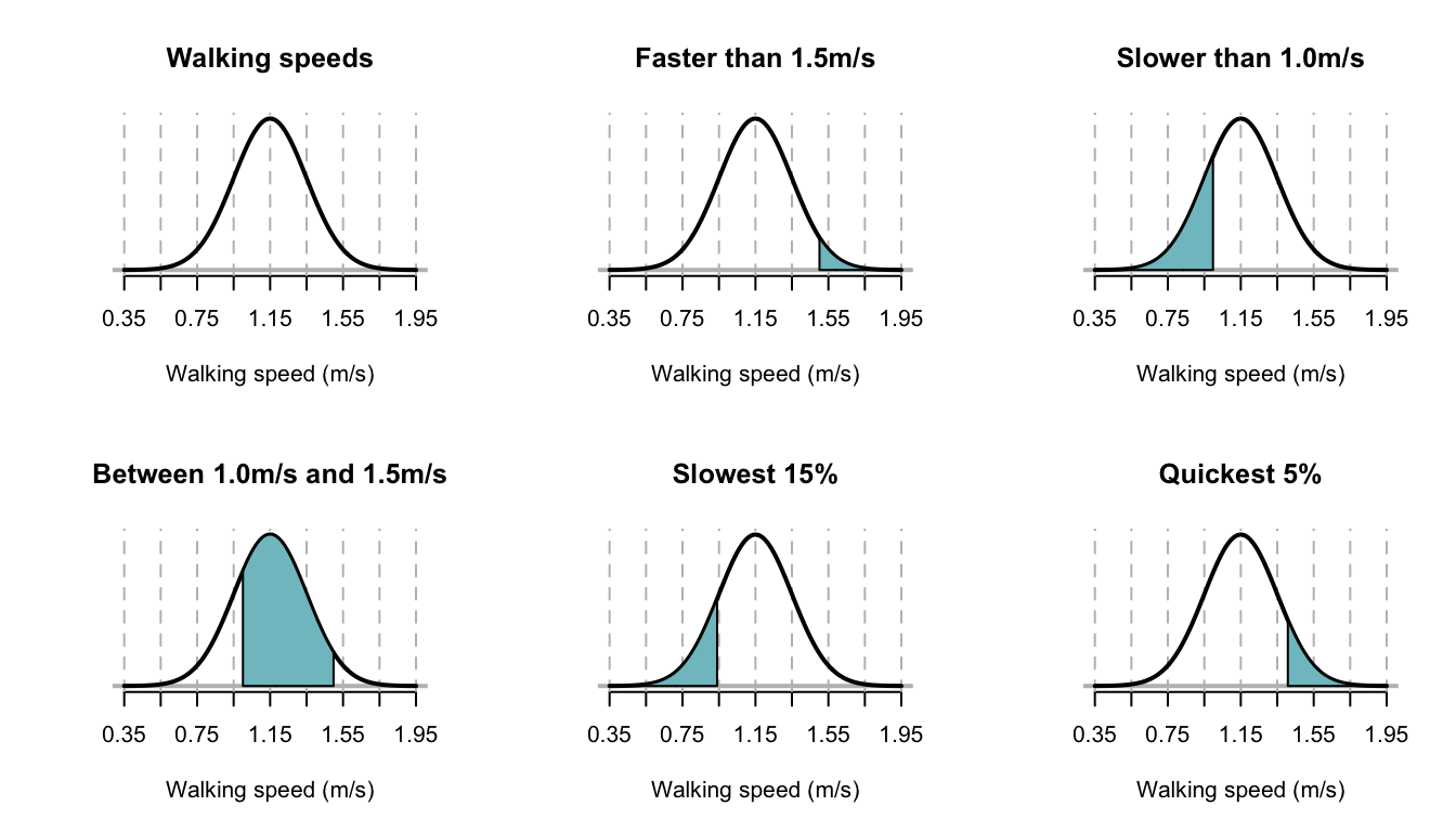
Figure 5.3: The normal distribution used for modelling walking speeds. The vertical dotted lines are at the mean and \(\pm1\), \(\pm2\), \(\pm3\) and \(\pm4\) standard deviations from the mean.

Example 5.3 (Using normal distributions) An examination has mean score of 500 and standard deviation 100. The top 75% of candidates taking this examination are to be passed. Assuming the score has a normal distribution, what is the lowest passing score?

We have \(X\sim N(500, 100^2)\). Let \(x_1\) be such that
\[\begin{align*} \Pr(X > x_1) &= 0.75\\ \Pr\left(Z > \frac{x_1 - 500}{100}\right) &= 0.75\\ \Pr\left(Z < \frac{500 - x_1}{100}\right) & = 0.75. \end{align*}\] From tables, \(0.75 = \Phi(0.675)\) so \((500 - x_1)/100 = 0.675\) and \(x_1 = 432.5\). Using R:

qnorm(0.25, # Top 75% = bottom 25% 
      mean = 500,
      sd = 100)
#> [1] 432.551

5.3.4 Normal approximation to the binomial

In Sect. 4.4, the binomial distribution was considered. Sometimes using the binomial distribution is tedious; consider a binomial random variable \(X\) where \(n = 1000\), \(p = 0.45\) and \(\Pr(X > 650)\) is sought: we would calculate \(\Pr(X = 651) + \Pr(X = 652) + \cdots + \Pr(X = 1000)\).

However, sometimes the normal distribution can be used to approximate binomial probabilities. For certain parameter values, the binomial pf starts to take on a normal distribution shape (Fig. 5.4).

When is the binomial pf close enough to use the normal approximation? There is no definitive answer; a common guideline suggests that if both \(np \ge 5\) and \(n(1 - p) \ge 5\) the approximation is satisfactory. (These are only guidelines, and other texts may suggest different guidelines.)

Figure 5.4 shows some picture of various binomial probabilty functions overlaid with the corresponding normal distribution; the approximation is visibly better as the guidelines given above are satisfied.

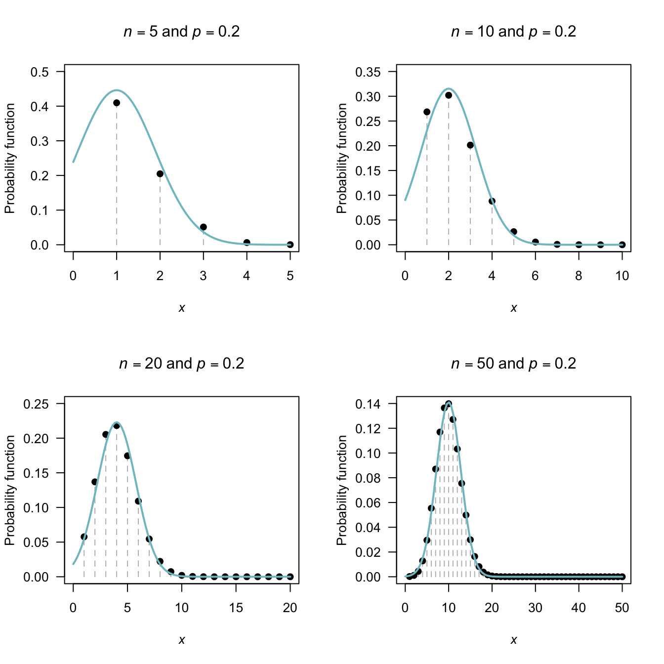
Figure 5.4: The normal distribution approximating a binomial distribution. The guidelines suggest the approximation should be good when \(np \ge 5\) and \(n (1 - p) \ge 5\); this is evident from the pictures. In the top row, a significant amount of the approximating normal distribution even appears when \(Y < 0\).

The normal distribution can be used to approximate probabilities in situations that are actually binomial. A fundamental difficulty with this approach is that a discrete distribution is being modelled with a continuous distribution. This is best explained through an example. The example explains the principle; the idea extends to all situations where the normal distribution is used to approximate a binomial distribution.

If the random variable \(X\) has the binomial distribution \(X \sim \text{Bin}(n, p)\), the probability function can be approximated by the normal distribution \(Y \sim \text{Norm}(\mu, \sigma^2)\), where \(\mu = np\) and \(\sigma^2 = np(1 - p)\).

The approximation is good if both \(np \ge 5\) and \(n(1 - p) \ge 5\).

Example 5.4 (Normal approximation to binomial) Consider mdx mice (which have a strain of muscular dystrophy) from a particular source for which \(30\)% of the mice survive for at least \(40\) weeks. One particular experiment requires at least \(35\) of the \(100\) mice to live beyond \(40\) weeks. What is the probability that \(35\) or more of the group will survive beyond \(40\) weeks?

First see that the situation is binomial; if \(X\) is the number of mice from the group of \(100\) that survive, then \(X \sim \text{Bin}(100, 0.3)\). This could be approximated by the normal distribution \(Y\sim N(30, 21)\), where the variance is \(np(1 - p) = 100\times 0.3\times 0.7 = 21\). Both \(np = 30\) and \(n(1 - p) = 70\) are much larger than \(5\), so this approximation is expected to adequate.

Figure 5.5 shows the upper tail of the distribution near \(X = 35\): using the normal approximation from \(Y = 35\), only half of the original bar in the binomial pf is included. However, since the number of mice is discrete, we want the entire bar corresponding to \(X = 35\). So to compute the correct answer, the normal distribution must be evaluated for \(\Pr(Y > 34.5)\). This change from \(Y \ge 34.5\) to \(Y > 34.5\) is called using the continuity correction.

The exact answer (using the binomial distribution) is \(0.1629\) (rounded to four decimal places). Using the normal distribution with the continuity correction gives the answer as \(0.1631\); using the normal distribution without the continuity correction, the answer is \(0.1376\). The solution is more accurate, as expected, using the continuity correction.

# Exact
ExactP <- sum( dbinom(x = 35:100,
                      size = 100,
                      prob = 0.30))
ExactP2 <- 1 - pbinom(34, 
                      size = 100,
                      prob = 0.30)
# Normal approx
NormalP <- 1 - pnorm(35, 
                     mean = 30,
                     sd = sqrt(21))
# Normal approx with continuity correction
ContCorrP <- 1 - pnorm(34.5, 
                       mean = 30,
                       sd = sqrt(21))
cat("Exact:" = round(ExactP, 6), "\n") # \n means "new line" 
#> 0.162858
cat("Exact (alt):" = round(ExactP2, 6), "\n")
#> 0.162858
cat("Normal approx:" = round(NormalP, 6), "\n")
#> 0.137617
cat("With correction:" = round(ContCorrP, 6), "\n")
#> 0.163055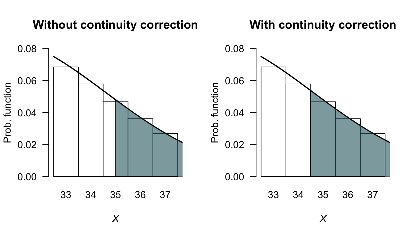

Figure 5.5: The normal distribution approximating the binomial distribution when \(n = 100\), \(p = 0.3\) and finding the probability that \(X > 35\).

Example 5.5 (Continuity correction) Consider rolling a standard die 100 times, and counting the number of times a appear uppermost. The random variable \(X\) is the number of times a appears; then, \(X\sim \text{Bin}(n = 100, p = 1/6)\).

Since \(np = 16.667\) and \(n(1 - p) = 83.333\) are both greater than \(5\), a normal approximation should be accurate, so define \(Y\sim N(16.6667, 13.889)\) (where the variance is \(np(1 - p) = 13.889\)). Various probabilities (Table 5.1) show the accuracy of the approximation, and the way in which the continuity correction has been used.

You should understand how the concept of the continuity correction has been applied in each situation, and be able to compute the probabilities for the normal approximation.

Table 5.1: Some events and their probabilities for the die-rolling example, computed using the binomial distribution (exact) and the normal approximation using the continuity correction. The accuracy of the approximation is generally very good.

Event (binomial)	Prob (binomial)		Event (normal)	Prob (normal)
\(\Pr(X \lt 10)\)	0.0213		\(\Pr(Y \lt 9.5)\)	0.0368
\(\Pr(X \le 15)\)	0.3877		\(\Pr(Y \lt 15.5)\)	0.3771
\(\Pr(X \gt 17)\)	0.4006		\(\Pr(Y \gt 17.5)\)	0.4115
\(\Pr(X \ge 21)\)	0.1519		\(\Pr(Y \gt 20.5)\)	0.1518
\(\Pr(15 \lt X \le 17)\)	0.2117		\(\Pr(15.5 \lt Y \lt 17.5)\)	0.2113

5.4 Exponential distribution

One shortcoming of using the normal distribution in modelling is that it is defined for all real values, but many quantities are defined on the positive real numbers only. This is not always a problem, especially when the observations are far from zero, such as heights of adult humans. However, many random variables have observations close to zero, and the data are often skewed to the right (positively skewed).

Many distributions can be used for modelling right-skewed data defined on the positive real numbers; the simplest is the exponential distribution.

5.4.1 Derivation

The exponential distribution is closely related to the Poisson distribution.

Consider a Poisson process, where events occur at an average rate of \(\lambda\) events per unit time (e.g., \(\lambda = 0.5\) per minute).

Then consider a fixed length of time \(t > 0\); then, the number of occurrences \(Y\) would have an average rate of \(\lambda t\) (e.g., in 12 minutes, we’d expect an average rate of \(0.5\times 12 = 6\) occurrences). That is, the number of events occurring in the interval \((0, t)\) has Poisson distribution with mean \(\lambda t\), with probability function
\[\begin{equation} p_Y(y) = \frac{\exp(-\lambda t) (\lambda t)^y}{y!} \quad \text{for $y = 0, 1, 2, \dots$}. \tag{5.9} \end{equation}\] Hence, the probability that zero events occur in the interval \((0, t)\) is
\[ \Pr(Y = 0) = \frac{\exp(-\lambda t) (\lambda t)^0}{0!} = \exp(-\lambda t) \] using \(Y = 0\) in (5.9).

Now, introduce a new random variable \(T\) that represent the time until the first event occurs. Then, \(Y = 0\) (i.e., no events occur in the interval \((0, t)\)) corresponds to \(T > t\) (i.e., the time till the first event occurs must be great than the time interval \(t\)). That is,
\[ \Pr(Y = 0) = \exp(-\lambda t) = \Pr(T > t). \] Rewriting in terms of a distribution function for \(T\),
\[ F_T(t) = 1 - \Pr(T > t) = 1 - \exp(-\lambda t) \] for \(t > 0\). Hence, the probability density function is
\[ f_T(t) = \lambda \exp(-\lambda t) \] for \(t > 0\). This is the probability density function for the exponential distribution.

This shows that if events occur at random according to a Poisson distribution, then the time (or the space) between those events follows an exponential distribution (Theorem 5.4). Hence the exponential distribution is used to describe the interval between consecutive randomly occurring events that follow a Poisson distribution.

Theorem 5.4 (Poisson process and exponential distributions) Consider a Poisson process at rate \(\lambda\) and suppose observation starts at an arbitrary time point. Then the time \(T\) to the first event has an exponential distribution with mean \(\text{E}(T) = 1/\lambda\); i.e.,
\[ f_T(t) = \lambda e^{-\lambda t},\quad t > 0. \]

Although the theorem refers to ‘time’, the variable of interest may be distance or any other continuous variable measuring the interval between events.

If events occur according to a Poisson distribution, then the “time” between the Poisson events can be modelled using an exponential distribution.

5.4.2 Definition and properties

The exponential distribution is usually written as follows.

Definition 5.8 (Exponential distribution) If a random variable \(X\) has the pdf
\[\begin{equation} f_X(x; \beta) = \displaystyle \frac{1}{\beta} \exp(-x/\beta) \quad \text{for $x > 0$} \tag{5.10} \end{equation}\] then \(X\) has an exponential distribution with parameter \(\beta > 0\). We write \(X\sim\text{Exp}(\beta)\).

The parameter \(\lambda = 1/\beta\) is often used in place of \(\beta\), and is called the rate parameter. Sometimes the notation \(X\sim\text{Exp}(\lambda)\), so checking which notation is being used in any context is wise. Plots of the pdf for various exponential distributions are given in Fig. 5.6}.

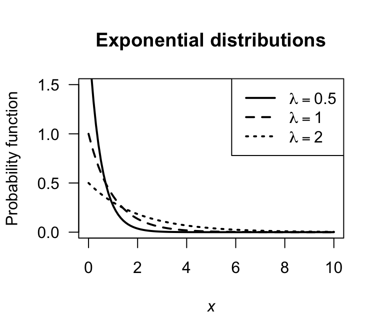
Figure 5.6: Exponential distributions for various values of the rate parameter \(\lambda = 1/\beta\)

Definition 5.9 (Exponential distribution: distribution function) For a random variable \(X\) with the exponential distribution given in (5.10), the distribution function is
\[ F_X(x; \lambda) = 1 - \exp\left\{-x/\beta\right\} = 1 - \exp\left\{-\lambda x\right\} \] for \(x > 0\).

The following are the basic properties of the exponential distribution.

Theorem 5.5 (Exponential distribution properties) If \(X\sim\text{Exp}(\beta)\) then

1. \(\text{E}(X) = \beta = 1/\lambda\).
2. \(\text{var}(X) = \beta^2 = 1/\lambda^2\).
3. \(M_X(t) = (1 - \beta t)^{-1}\) for \(t < 1/\beta\) (or, \(M_X(t) = \lambda/(\lambda - t)\) for \(t < \lambda\)).

Proof. The proofs are left as an exercise.

The parameter \(\beta\) represents the mean of the exponential distribution. The alternative parameter \(\lambda = 1/\beta\) represents the mean rate at which events occur. Like the Poisson distribution, the variance is defined once the mean is defined .

The four R functions for working with the exponential distribution have the form [dpqr]exp(rate) where rate\({}= \lambda = 1/\beta\) (see Appendix B).

Example 5.6 (Exponential distributions) Allen et al. (1975) use the exponential distribution to model daily rainfall in Kentucky.

Example 5.7 (Exponential distributions) Cox and Lewis (1966) give data collected by Fatt and Katz concerning the time intervals between successive nerve pulses along a nerve fibre. There are 799 observations which we do not give here. The mean time between pulses is \(\beta = 0.2186\) seconds. An exponential distribution might be expected to model the data well. This is indeed the case (Fig. 5.7). What proportion of time intervals can be expected to be longer than 1 second?

If \(X\) is the time between successive nerve pulses (in seconds), then \(X\sim \text{Exp}(\beta = 0.2186)\) (so the rate parameter is \(\lambda = 1/0.2186 = 4.575\) per second). The solution will then be
\[\begin{align*} \Pr(X > 1) &= \int_1^\infty \frac{1}{0.2186}\exp(-x/0.2186)\, dx \\ &= -\exp(-x/0.2186)\Big|_1^\infty \\ &= (-0) + (\exp\{-1/0.2186\})\\ &= 0.01031. \end{align*}\] There is about a 1% chance of a nerve pulse exceeding one second.

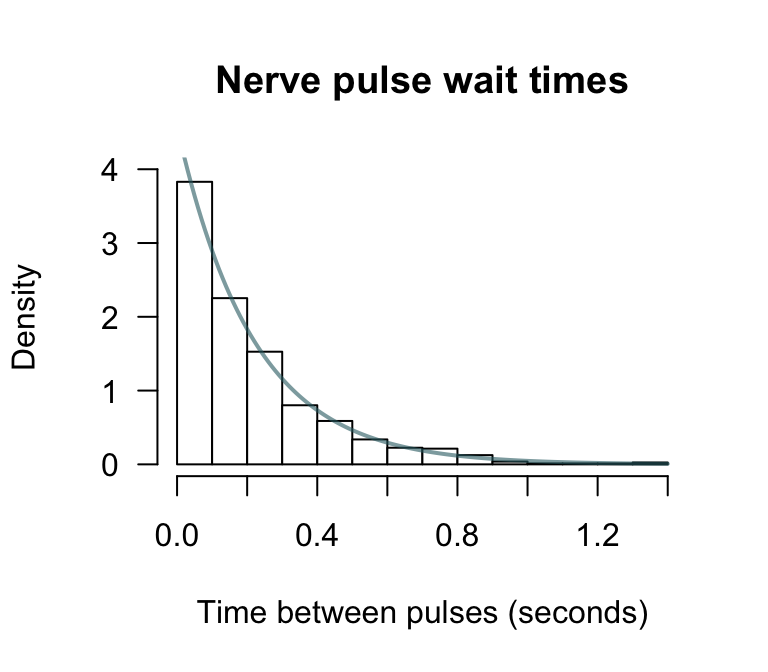
Figure 5.7: The time between successive nerve pulses. An exponential distribution fits well.

The relationship between the Poisson and exponential distribution was explored in Sect. 5.4.1 (see, for example, Theorem 5.4). The next example explores this relationship

Example 5.8 (Relationship between exponential and Poisson distributions) Suppose a Poisson process occurs at the mean rate of 5 events per hour. Let \(N\) represent the number of events in one day and \(T\) the time between consecutive events. We can describe the distribution of the time between consecutive events and the distribution of the number of events in one day (24 hours).

Since events occur at the mean rate of \(\lambda = 5\) events per hour, the mean time between consecutive events is \(\beta = 1/\lambda = 0.2\) hours. Hence, the mean number of events in one day is \(\mu = 24\times 5 = 120\).

Consequently, \(N\sim\text{Pois}(\mu = 120)\) and \(X\sim\text{Exp}(\beta = 0.2)\) (or, equivalently, \(X\sim\text{Exp}(\lambda = 5)\)).

An important feature of a Poisson process, and hence of the exponential distribution, is the memoryless or Markov property: the future of the process at any time point does not depend on the history of the process. This property is captured in the following theorem.

Theorem 5.6 (Memoryless property) If \(T \sim \text{Exp}(\lambda)\) where \(\lambda\) is the rate parameter, then for \(s > 0\) and \(t > 0\),
\[ \Pr(T > s + t \mid T > s) = \Pr(T > t) \]

Proof. Using Definition 1.12,
\[ \Pr(T > s + t \mid T > s) = \frac{ \Pr( \{T > s + t\} \cap \{T > s\})} {\Pr(T > s)} \] But if \(T > s + t\), then \(T > s\). Consequently \(\Pr( \{T > s + t \}\cap \{T > s \} ) = \Pr(T > s + t)\) and so
\[\begin{align*} \Pr(T > s + t \mid T > s ) &= \frac{\Pr(T > s +t )}{\Pr(T > s)}\\ &= \frac{\exp\left\{-\lambda(s + t)\right\}}{\exp\left\{-\lambda s\right\}}\\ &= \exp\left\{-\lambda t\right\}\\ &= \Pr(T > t). \end{align*}\]

This theorem states that the probability that the time to the next event is greater than \(t\) does not depend on the time \(s\) back to the previous event. This is called the memoryless property of the exponential distribution.

Example 5.9 (Memoryless property of exponential distribution) Suppose the lifespan of component \(A\) is modelled by an exponential distribution with mean 12 months. Then, \(T \sim \text{Exp}(\beta = 6)\).

The probability that component \(A\) fails in less than 6 months is
\[ \Pr(T < 6) = 1 - \exp(-6/12) = 0.3935. \]

Now, suppose component \(A\) has been in place for 12 months. The probability that it will fail in less than a further 6 months is
\[ \Pr(T < 18 | T > 12) = \Pr(T < 6) = 1 - \exp(-6/12) = 0.3935 \] by the memoryless property.

Example 5.9 shows that an exponential process is ‘ageless’: the risk of ‘mortality’ remains constant with age. That is, the probability of such an event occurring in the next small interval, whether the failure of a component or the occurrence of an accident, remains constant regardless of the age of the component or the length of time since the last accident. In this sense, an exponential lifetime is different from a human lifetime, or the lifetime of many man-made objects, where the risk of ‘death’ in the next small interval increases with age.

5.5 Gamma distribution

Once the mean of an exponential distribution is defined, the variance is defined. More flexibility is sometimes needed, which is provided by the gamma distribution.

Definition 5.10 (Gamma distribution) If a random variable \(X\) has the pdf
\[ f_X(x; \alpha, \beta) = \frac{1}{\beta^\alpha \Gamma(\alpha)} x^{\alpha - 1} \exp(-x/\beta) \] then \(X\) has a gamma distribution, where \(\Gamma(\cdot)\) is the gamma function (see Sect. 4.11) and \(\alpha, \beta > 0\). We write \(X \sim \text{Gam}(\alpha, \beta)\).

The parameter \(\alpha\) is called the shape parameter and \(\beta\) is called the scale parameter. Some texts use different notation for the shape and scale parameters. In broad terms, the shape parameter dictates the general shape of the distribution; the scale parameter dictates how ‘stretched out’ the distribution is.

In R, the gamma function \(\Gamma(x)\) is evaluated using gamma(x).

The four R functions for working with the gamma distribution have the form [dpqr]gamma(shape, rate, scale = 1/rate), where shape\({}= \alpha\) and scale\({}= \beta\) (see Appendix B).

Plots of the gamma pdf for various values of the parameters are given in Fig. 5.8. In the bottom right panel, the gamma distributions are starting to look a bit like normal distributions.

The exponential distribution is a special case of the gamma distribution with \(\alpha = 1\). This means that properties of the exponential distribution can be obtained by substituting \(\alpha = 1\) into the formulae for the gamma distribution.

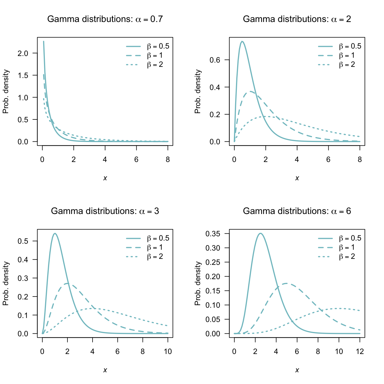
Figure 5.8: The pdf of a gamma distribution for various values of \(\alpha\) and \(\beta\)

Notice that
\[\begin{align} \int_0^\infty f_X(x)\,dx &= \int_0^\infty\frac{e^{-x/\beta}x^{\alpha - 1}}{\beta^\alpha\Gamma(\alpha)}\,dx\nonumber\\ &= \frac{1}{\Gamma(\alpha)} \int_0^\infty e^{-y} y^{\alpha-1}\,dy \quad \text{(on putting $y = x/\beta$)}\nonumber \\ &= 1, \tag{5.11} \end{align}\] because \(\int_0^\infty \exp(-y) y^{\alpha-1}\,dy = \Gamma(\alpha)\).

The distribution function for the gamma distribution is complicated, involving incomplete gamma functions, and will not be given. The following are the basic properties of the gamma distribution.

Theorem 5.7 (Gamma distribution properties) If \(X\sim\text{Gam}(\alpha,\beta)\) then

1. \(\text{E}(X) = \alpha\beta\).
2. \(\text{var}(X) = \alpha\beta^2\).
3. \(M_X(t) = (1-\beta t)^{-\alpha}\) for \(t < 1/\beta\).

Proof. For the expected value:
\[ \text{E}(X) = \int_0^{\infty}x f_X(x)\,dx = \beta \frac{\Gamma(\alpha + 1)}{\Gamma(\alpha)} \underbrace{\int_0^{\infty}\frac{\exp(-x/\beta) x^{(\alpha + 1) - 1}}{\beta^{\alpha + 1}\Gamma(\alpha + 1)} \, dx}_{= 1} = \alpha\beta. \] This result follows from using (5.11) and Theorem 5.7
\[ \text{E}(X^2) = \int_0^{\infty}x^2 f_X(x) \, dx = \beta^2\frac{\Gamma(\alpha + 2)}{\Gamma(\alpha)} \underbrace{\int_0^{\infty}\frac{\exp(-x/\beta) x^{(\alpha + 2) - 1}}{\beta^{\alpha + 2}\Gamma(\alpha + 2)}\,dx}_{= 1} = \alpha(\alpha + 1)\beta^2 \] where the result follows by writing \(\Gamma(\alpha + 2) = (\alpha + 1)\alpha\Gamma(\alpha)\). Hence
\[ \text{var}(X) = \text{E}(X^2) - [\text{E}(X)]^2 = \alpha(\alpha + 1)\beta^2 - (\alpha\beta)^2 = \alpha\beta^2 \] Also:
\[\begin{align*} M_X(t) = \text{E}(e^{Xt}) &= \int_0^{\infty}\exp(tx) \frac{\exp(-x/\beta) x^{\alpha - 1}}{\beta^{\alpha} \Gamma(\alpha)} \, dx\\ &= \int_0^{\infty} \frac{\exp\{-x(1 - \beta t)/\beta\}x^{\alpha - 1}}{\beta^{\alpha}\Gamma(\alpha)} \, dx\\ &= \int_0^{\infty} \frac{\exp(-z) z^{\alpha - 1}}{\Gamma(\alpha)(1 - \beta t)^{\alpha - 1}} \, \frac{dz} {1 - \beta t}, \text{putting $z = x(1 - \beta t)/\beta$}\\ &= (1 - \beta t)^{-\alpha}, \end{align*}\] since the integral remaining is 1.

As usual the moments can be found by expanding \(M_X(t)\) as a series. That is,
\[ M_X(t) = 1 \ + \ \alpha\beta t \ + \ \frac{\alpha(\alpha+1)\beta^2}{2!} t^2 \ + \ \cdots \] from which
\[\begin{align*} E(X) &= \text{coefficient of }t =\alpha\beta,\\ E(Y^2) &= \text{coefficient of }t^2/2!=\alpha(\alpha+1)\beta^2, \end{align*}\] as found earlier.

As for the normal distribution, the distribution function of the gamma cannot, in general, be computed without using numerical integration, tables (although see Example 5.11) or software.

Example 5.10 (Rainfall) Das (1955) used a (truncated) gamma distribution for modelling daily precipitation in Sydney. A similar approach is adopted by (D. S. Wilks 1990).

Larsen and Marx (1986) (Case Study 4.6.1) use the gamma distribution to model daily rainfall in Sydney, Australia using the parameter estimates \(\alpha = 0.105\) and \(\beta = 76.9\) (based on Das (1955)). The comparison between the data and the model (Table 5.2) indicates a good agreement between the data and the theoretical distribution.

Table 5.2: The gamma distribution used to model Sydney daily rainfall

Rainfall (mm)	Observed	Modelled		Rainfall (mm)	Observed	Modelled
0–5	1631	1639		46–50	18	12
6–10	115	106		51–60	18	20
11–15	67	62		61–70	13	15
16–20	42	44		71–80	13	12
21–25	27	32		81–90	8	9
26–30	26	26		91–100	8	7
31–35	19	21		101–125	16	12
36–40	14	17		126–150	7	7
41–45	12	14		151–425	14	13

Example 5.11 (Electrical components) The lifetime of an electrical component in hours, say \(T\), can be well modelled by the distribution \(\text{Gam}(2, 1)\). What is the probability that a component will last for more than three hours?

From the information, \(T\sim \text{Gam}(\alpha = 2, \beta = 1)\). The required probability is therefore
\[\begin{align*} \Pr(T > 3) &= \int_3^\infty \frac{1}{1^2 \Gamma(2)}t^{2 - 1} \exp(-t/1)\,dt \\ &= \int_3^\infty t \exp(-t)\,dt \\ \end{align*}\] since \(\Gamma(2) = 1! = 1\). This expression can be integrated using integration by parts:
\[\begin{align*} \Pr(T > 3) &= \int_3^\infty t \exp(-t)\,dt \\ &= \left\{ -t \exp(-t)\right\}\Big|_3^\infty - \int_3^\infty -\exp(-t)\, dt \\ &= [ (0) - \{-3\exp(-3)\}] - \left\{ \exp(-t)\Big|_3^\infty\right\} \\ &= 3\exp(-3) + \exp(-3)\\ &= 0.1991 \end{align*}\]

Integration by parts is only possible since \(\alpha\) is integer. If \(\alpha\) was, for example \(\alpha = 2.5\), integration by parts would not be possible.

A more general approach is to use tables of the incomplete gamma function to evaluate the integral, numerical integration, or software. To use R:

# Integrate
integrate(dgamma, # The gamma distribution prob. fn
          lower = 3,
          upper = Inf,  # "Inf" means "infinity"
          shape = 2,
          scale = 1)
#> 0.1991483 with absolute error < 9.3e-05

# Directly
1 - pgamma(3,
           shape = 2,
           scale = 1)
#> [1] 0.1991483

Using any method, the probability is about 20%.

Example 5.12 (Gamma) If \(X\sim \text{Gam}(\alpha, \beta)\), find the distribution of \(Y = kX\) for some constant \(k\).

One way to approach this question is to use moment-generating functions. Since \(X\) has a gamma distribution, \(M_X(t) = (1-\beta t)^{-\alpha}\). Now,
\[\begin{align*} M_Y(t) &= \text{E}(\exp(tY)) \qquad\text{by definition of the mgf}\\ &= \text{E}(\exp(t kX)) \qquad\text{since $X = kX$}\\ &= \text{E}(\exp(s X)) \qquad\text{by letting $s = kt$}\\ &= M_X(s) \qquad\text{by definition of the mgf}\\ &= M_X(kt) \\ &= (1 - \beta kt)^{-\alpha}. \end{align*}\] This is just the mgf for random variable \(X\) with \(k\beta\) in place of \(\beta\), so the distribution of \(Y\) is \(\text{Gam}(\alpha, k\beta)\).

5.6 Beta distribution

Some continuous random variables are constrained to a finite interval. The beta distribution is useful in these situations.

Definition 5.11 (Beta distribution) A random variable \(X\) with probability density function
\[\begin{equation*} f_X(x; m, n) = \frac{x ^ {m - 1}(1 - x)^{n - 1}}{B(m, n)} \quad \text{for $0\leq x \leq 1$ and $m > 0$, $n > 0$}, \end{equation*}\] and \(B(m, n)\) is the beta function
\[\begin{align} B(m, n) &= \int_0^1 x^{m - 1}(1 - x)^{n - 1} \, dx, \quad \text{for $m > 0$ and $n > 0$}\nonumber\\ &= \frac{\Gamma(m)\, \Gamma(n)}{\Gamma(m + n)}, \tag{5.12} \end{align}\] is said to have a beta distribution with parameters \(m\) and \(n\). We write \(X \sim \text{Beta}(m, n)\).

\(B(m, n)\) defined by (5.12) is known as the beta function with parameters \(m\) and \(n\). Since \(\int_0^1 f_X(x)\,dx = 1\) then
\[\begin{equation} \int_0^1 \frac{x^{m - 1}(1 - x)^{n - 1}}{B(m, n)}\,dx = 1. \end{equation}\]

In R, the beta function is evaluated using beta(a, b), where a\({} = m\) and b\({} = n\).

The four R functions for working with the beta distribution have the form [dpqr]beta(shape1, shape2), where shape1\({}= m\) and shape2\({}= n\) (see Appendix B).

The distribution function for the beta distribution is complicated, involving incomplete beta functions, and will not be given. Some properties of the beta function follow.

Theorem 5.8 (Beta function properties) The beta function (5.12) satisfies the following:

1. The beta function is symmetric in \(m\) and \(n\). That is, if \(m\) and \(n\) are interchanged, the function remains unaltered; i.e., \(B(m, n) = B (n, m)\).
2. \(B(1, 1) = 1\).
3. \(B\left(\frac{1}{2}, \frac{1}{2}\right) = \pi\).

Proof. To prove the first, put \(z = 1 - x\) and hence \(dz = -dx\) in (5.12). Then
\[\begin{align*} B(m, n) &= -\int_1^0(1 - z)^{m - 1} z^{n - 1} \, dz\\ &= \int_0^1 z^{n - 1}(1 - z)^{m - 1} \, dz\\ &= B(n, m). \end{align*}\]

For the second, put \(x = \sin^2\theta\), and so \(dx = 2\sin\theta\cos\theta\,d\theta\), in (5.12). We have
\[ B(m, n) = 2 \int_0^{\pi/2} \sin^{2m - 1}\theta \cos ^{2n - 1}\theta\,d\theta. \] So, for \(m = n = \frac{1}{2}\),
\[ B\left(\frac{1}{2}, \frac{1}{2}\right) = 2\int_0^{\pi/2} d\theta = \pi. \]

For the third, note that \(\Gamma(1/2) = \sqrt{\pi}\) from Theorem 5.7. Further, since \(\Gamma(1) = 0! = 1\), the results follows.

Typical graphs for the beta pdf are given in Fig. 5.9. When \(m = n\), the distribution is symmetric about \(x = \frac{1}{2}\).

When \(m = n = 1\), the beta distribution becomes the uniform distribution on \((0, 1)\).

Figure 5.9: Various beta-distribution pdfs

Some basic properties of the beta distribution follow.

Theorem 5.9 (Beta distribution properties) If \(X \sim \text{Beta}(m, n)\) then

1. \(\text{E}(X) = m/(m + n)\).
2. \(\displaystyle\text{var}(X) = \frac{mn}{(m + n)^2 (m + n + 1)}\).
3. A mode occurs at \(\displaystyle x = \frac{m - 1}{m + n - 2}\) for \(m, n > 1\).

Proof. Assume \(X \sim \text{Beta}(m, n)\), then
\[\begin{align*} \mu_r' =\text{E}(X^r) &= \int_0^1 \frac{x^r x^{m - 1}(1 - x)^{n - 1}} {B(m, n)}\,dx\\ &= \frac{B(m + r, n)}{B(m, n)} \int_0^1 \frac{x^{m + r - 1}(1 - x)^{n - 1}}{B(m + r, n)}\,dx\\ &= \frac{\Gamma(m + r)\,\Gamma(n)}{\Gamma(m + r + n)} \frac{\Gamma(m + n)}{\Gamma(m)\,\Gamma(n)}\\ &= \frac{\Gamma(m + r)\,\Gamma(m + n)}{\Gamma(m + r + n)\,\Gamma(m)} \end{align*}\] Putting \(r = 1\) and \(r = 2\) into the above expression, and using that \(\text{var}(X) = \text{E}(X^2) - \text{E}(X)^2\), the mean and variance are \(\text{E}(X) = m/(m + n)\) and \(\text{var}(X) = \frac{mn}{(m + n)^2(m + n + 1)}\).

Any mode \(\theta\) of the distribution for which \(0 < \theta < 1\) will satisfy \(f'_X(\theta) = 0\). From the definition we see that for \(m, n>1\) and \(0 < x < 1\),
\[ f'_X(x) = (m - 1)x^{m - 2} (1 - x)^{n - 1} - (n - 1)x^{m - 1}(1 - x)^{n - 1}/B(m, n) = 0 \] implying \((m - 1)(1 - x) = (n - 1)x\) which is satisfied by \(x = (m - 1) / (m + n - 2)\).

The mgf of the beta distribution cannot be written in terms of standard functions. The distribution function of the beta must be evaluated numerically in general, except when \(m\) and \(n\) are integers as shown in the example below.

If \(X\sim \text{Beta}(m, n)\), then \(X\) is defined on \([0, 1]\). Sometimes then, the beta distribution is used to model proportions, though not proportions out of a total number (when the binomial distribution is used). Instead, the beta distribution is used, for example, to model percentage cloud cover (for example, Falls (1974)).

For a random variable \(Y\) defined on a different closed interval \([a, b]\), define \(Y = X(b - a) + a\).

Example 5.13 Damgaard and Irvine (2019) use the beta-distribution to model the relative areas covered by plants of different species. The beta distribution is a suitable model, since these relative areas are proportions. In addition, the authors state that

…plant cover data tend to be left-skewed (J-shaped), right skewed (L-shaped) or U-shaped (p. 2747)

which align with some of the plots in Fig. 5.9.

Example 5.14 (Beta distributions) The bulk storage tanks of a fuel retailed are filled each Monday. The retailer has observed that over many weeks the proportion of the available fuel supply sold is well modelled by a beta distribution with \(m = 4\) and \(n = 2\).

If \(X\) denotes the proportion of the total supply sold in a given week, the mean proportion of fuel sold each week is
\[ \text{E}(X) = m/(m + n) = 4/6 = 2/3. \]

To find the probability that at least 90% of the supply will sell in a given week, compute:
\[\begin{align*} \Pr(X > 0.9) &= \int_{0.9}^1\frac{\Gamma(4 + 2)}{\Gamma(4)\Gamma(2)}x^3(1 - x)dx\\ &= 20\int_{0.9}^1 (x^3 - x^4))\,dx\\ &= 20(0.004)\\ &= 0.08 \end{align*}\] It is unlikely that 90% of the supply will be sold in a given week. In R:

1 - pbeta(0.9, 
          shape1 = 4, 
          shape2 = 2)
#> [1] 0.08146

5.7 Simulation

As with discrete distributions (Sect. 4.9), simulation can be used with continuous distributions. Again, in R, random numbers from a specific distribution use functions that start with the letter r; for example, to generate random numbers from a normal distribution, use rnorm():

rnorm(3, # Generate three random numbers...
      mean = 4,     # ... with mean = 4
      sd = 2)       # ... with sd = 2
#> [1] 1.748524 4.082457 2.624341

Suppose we are seeking women over 173cm tall for a study; what percentage of women are over 173cm tall? Assume that adult females have heights modelled by a normal distribution with mean 163cm and a standard deviation of 5cm (Australian Bureau of Statistics 1995). The percentage taller than 173 cm is:

1 - pnorm(173, mean = 163, sd = 5)
#> [1] 0.02275013

Simulations can also be used, which allows us to consider more complex situations. For this simple question initially (Fig. 5.10, left panel):

htW <- rnorm(1000,  # One thousand women
             mean = 163,  # Mean ht
             sd = 5)      # Sd of height
pcTallWomen <- sum( htW > 173 )/1000 * 100

cat("Percentage 'tall' women:", pcTallWomen, '%\n')
#> Percentage 'tall' women: 2.3 %

Now consider a more complex situation. Suppose adult males have heights with a mean of 175cm with standard deviation of 7cm, and constitute 44% of the population. Now, we are seeking women or men over 173cm tall (Fig. 5.10, right panel):

personSex <- rbinom(1000,  # Select sex of each person
                    1,
                    0.44) # So 0 = Male; 1 = Female

htP <- rnorm(1000,  # change ht parameters according to sex
             mean = ifelse(personSex == 0,
                           175,
                           163),
             sd = ifelse(personSex == 0,
                         7, 
                         5))

pcTallPeople <- sum( htP > 173 )/1000 * 100
pcFemales <- sum( personSex == 1 ) / 1000 * 100

cat("Percentage 'tall' people:", pcTallPeople, '%\n\n')
#> Percentage 'tall' people: 34.8 %
cat("Percentage females:", pcFemales, '%\n\n')
#> Percentage females: 43.2 %
cat("Percentage of 'tall' people that are female:", 
    round( sum(htP > 173 & personSex == 1) / sum(htP > 173) * 100, 1),
    '%\n\n')
#> Percentage of 'tall' people that are female: 2.6 %
cat("Variance of heights: ", var(htP), "\n")
#> Variance of heights:  71.09267

Figure 5.10: The distribution of heights of women (left panel) and men and women combined (right panel)

5.8 Exercises

Exercise 5.1 Write the beta distribution parameters \(m\) and \(n\) in terms of the mean and variance.

Exercise 5.2 In a study modelling pedestrian road-crossing behaviour (Shaaban and Abdel-Warith 2017), the uniform distribution is used in the simulation to model the vehicle speeds. The speeds have a minimum value of 30 km/h, and a maximum value of 72 km/h.

1. Using this model, compute the mean and standard deviation of vehicle speeds.
2. Compute and plot the pdf and df.
3. If \(X\) is the vehicle speed, compute \(\Pr(X > 60)\), where 60 km/h is the posted speed limit.
4. Compute \(\Pr(X > 65\mid X > 60)\).

Exercise 5.3 In a study modelling pedestrian road-crossing behaviour (Shaaban and Abdel-Warith 2017), the normal distribution is used in the simulation to model the vehicle speeds. The normal model has a mean of 48km/h, with a standard deviation² of 8.8km/h.

1. The article ignores all vehicles travelling slower than 30 km/h and faster than 72 km/h. What proportion of vehicles are excluded using this criterion?
2. Write the pdf for this truncated normal distribution.
3. Plot the pdf and df for this truncated normal distribution.
4. Compute the mean and variance for this truncated normal distribution.
5. Suppose a vehicle is caught speeding (i.e., exceeding 60 km/h); what is the probability that the vehicle is exceeding the speed limit by less than 5 km/h?

Exercise 5.4 A study of the service life of concrete in various conditions (Liu and Shi 2012) modelled the diffusion coefficients using a gamma distribution, with \(\alpha = 27.05\) and \(\beta = 1.42\) (units not given).

1. Plot the pdf and df.
2. Determine the mean and standard deviation of the chloride diffusion coefficients that were used in the simulation.
3. If \(C\) represents the chloride diffusion coefficients, compute \(\Pr(C > 30\mid C < 50)\).

Exercise 5.5 A study of the service life of concrete in various conditions (Liu and Shi 2012) used normal distributions to model the surface chloride concentrations. In one model, the mean was set as \(\mu = 2\) kg/m³ and the standard deviation as \(\sigma = 0.2\) kg/m³.

1. Plot the pdf and df.
2. Let \(Y\) be the surface chloride concentration. Compute \(\Pr(Y > 2.4)\).
3. 80% of the time, surface chloride concentrations are below what value?
4. 15% of the time, surface chloride concentrations exceed what value?

Exercise 5.6 An alternative to the beta distribution with a closed form is the Kumaraswamy distribution, with pdf
\[ p_X(x) = \begin{cases} ab x^{a - 1} (1 - x^a)^{b - 1} & \text{for $0 < x < 1$};\\ 0 & \text{elsewhere} \end{cases} \] for \(a > 0\) and \(b > 0\). We write \(X\sim \text{Kumaraswamy}(a, b)\).

1. Plot some densities for the Kumaraswamy distribution showing its different shapes.
2. Show that the df is \(F_X(x) = 1 - (1 - x^a)^b\) for \(0 < x < 1\). Plot the distribution functions corresponding to the pdfs in Part 1.
3. If \(X\sim \text{Kumaraswamy}(a, 1)\), then show that \(X\sim \text{Beta}(a, 1)\).
4. If \(X\sim \text{Kumaraswamy}(1, 1)\), then show that \(X\sim \text{Unif}(0, 1)\).
5. If \(X\sim \text{Kumaraswamy}(a, 1)\), then show that \((1 - X) \sim \text{Kumaraswamy}(1, a)\).

Exercise 5.7 Show that the gamma distribution has a constant coefficient of variation, where the coefficient of variation is the standard deviation divided by the mean.

Exercise 5.8 In a study modelling waiting times at a hospital (Khadem et al. 2008), patients are classified into one of three categories:

• Red: Critically ill or injured patients.
• Yellow: Moderately ill or injured patients.
• Green: Minimally injured or uninjured patients.

For ‘Green’ patients, the service time \(S\) was modelled as \(S = 4.5 + 11V\), where \(V \sim \text{Beta}(0.287, 0.926)\).

1. Find the mean and standard deviation of the service times \(S\).
2. Produce well-labelled plots of the pdf and df of \(V\), showing important features.

Exercise 5.9 In a study modelling waiting times at a hospital (Khadem et al. 2008), patients are classified into one of three categories:

• Red: Critically ill or injured patients.
• Yellow: Moderately ill or injured patients.
• Green: Minimally injured or uninjured patients.

The time (in minutes) spent in the reception are for ‘Yellow’ patients, say \(T\), is modelled as \(T = 0.5 + W\), where \(W\sim \text{Exp}(\beta = 16.5)\).

1. Find the mean and standard deviation of the waiting times \(T\).
2. Plot the pdf and df of \(W\).

Exercise 5.10 In a study modelling waiting times at a hospital (Khadem et al. 2008), patients are classified into one of three categories:

• Red: Critically ill or injured patients.
• Yellow: Moderately ill or injured patients.
• Green: Minimally injured or uninjured patients.

The time (in minutes) spent in the reception are for ‘Green’ patients, say \(T\), is modelled as a normal distribution with mean \(\mu = 45.4\) min and standard deviation \(\sigma = 23.4\) min.

1. Find the mean and standard deviation of the waiting times \(T\).
2. Plot the pdf and df of \(T\).
3. What proportion of ‘Green’ patients wait longer than an hour?
4. How long to the slowest \(10\)% of patients need to wait?

Exercise 5.11 In a study of rainfall (Watterson and Dix 2003), rainfall on wet days in SE Australia (37^\(\circ\)S; 146^\(\circ\)E) was simulated using a gamma distribution with \(\alpha = 0.62\) and \(\beta = 7.1\)mm.

1. Rainfall below \(0.0017\)mm cannot be recorded by the equipment used. What proportion of days does this represent?
2. Plot the pdf and df.
3. What is the probability that more than 3mm falls on a wet day?
4. The proportion of wet days is \(0.43\). What proportion of all days receive more than 3mm?

Exercise 5.12 In a study of rainfall disaggregation (Connolly, Schirmer, and Dunn 1998) (extracting small-scale rainfall features from large-scale measurements), the duration (in fractions of day) of non-overlapping rainfall events per day at Katherine was modelled using a Gamma distribution with \(\alpha = 2\), and \(\beta = 0.04\) in summer and \(\beta = 0.03\) in winter.

Denote the duration of rainfall events, in fractions of a day, be denoted in summer as \(S\), and in winter as \(W\).

1. Plot the rainfall event duration distributions, and compare summer and winter.
2. What is the probability of a rainfall event lasting more than 6 hours in winter?
3. What is the probability of a rainfall event lasting more than 6 hours in summer?
4. Describe what is meant by the statement \(\Pr(S > 3/24 \mid S > 1/24)\), and compute the probability.
5. Describe what is meant by the statement \(\Pr(W < 2/24 \mid W > 1/24)\), and compute the probability.

Exercise 5.13 In a study of rainfall disaggregation (Connolly, Schirmer, and Dunn 1998) (extracting small-scale rainfall features from large-scale measurements), the starting time of the first rainfall event at Katherine each day (scaled from 0 to 1) was modelled using a beta distribution with parameters \((1.16, 1.50)\) in summer and \((0.44, 0.56)\) in winter.

Denote the number of rainfall events in summer as \(S\), and in winter as \(W\).

1. Plot the two starting-time distributions, and compare summer and winter.
2. Compute the mean and standard deviation of starting times for both seasons.
3. What is the probability that the first rain event in winter is after 6am?
4. What is the probability that the first rain event in summer is after 6am?
5. Describe what is meant by the statement \(\Pr(S > 3 \mid S > 1)\), and compute the probability.
6. Describe what is meant by the statement \(\Pr(W > 2 \mid W > 1)\), and compute the probability.

Exercise 5.14 A study of the impact of diarrhoea (Schmidt, Genser, and Chalabi 2009) used a gamma distribution to model the duration of symptoms. In Guatemala, duration (in days) was modelled using a gamma distribution with \(\alpha = 1.11\) and \(\beta = 3.39\). Let \(X\) refer to the duration of symptoms.

1. Compute the mean and standard deviation of the duration.
2. The value of \(\alpha\) is close to one. Plot the pdf of the gamma distribution and the near-equivalent exponential distribution, and comment.
3. Compute \(\Pr(X > 4)\) using both the gamma and exponential distributions, and comment.
4. The patients in the 5% with symptoms the longest had symptoms for how long? Again, compare both models, and comment.

Exercise 5.15 In a study of office occupancy at a university (Luo et al. 2017), the leaving-times of professors were modelled as a normal distribution, with a mean leaving time of 6pm, with a standard deviation of 1.5h.

1. Using this model, what proportion of professors leave before 5pm?
2. Suppose a professor is still at work at 5pm; what is the probability that the professor leaves after 7pm?
3. The latest-leaving 15% of professors leave after what time?

Exercise 5.16 The percentage of clay content in soil has been modelled using a beta distribution. In one study (Haskett, Pachepsky, and Acock 1995), two counties in Iowa were modelled with beta-distributions: County A with parameters \(m = 11.52\) and \(n = 4.75\), and County B with parameters \(m = 3.85\) and \(n = 3.65\).

1. Plot the two distributions, and comment (in context).
2. Compute the mean and standard deviation of each county.
3. What percentage of soil samples exceed 50% clay in the two counties? Comment.

Exercise 5.17 A study of water uptake in plants in grasssland and savanna ecosystems (Nippert and Holdo 2015) used a beta distribution to model the distribution of root depth \(D\). The MRD (maximum root density) was 70cm, so the beta distribution used was defined over the interval \([0, 70]\). For one simulation, the beta-distribution parameters were \(m = 1\) and \(n = 5\).

1. Plot the pdf, and explain what it means in this context.
2. Determine the probability that the root depth was deeper than 50cm.
3. Determine the root depth of the plants with the deepest 20% of roots.

Exercise 5.18 Suppose that the measured voltage in a certain electrical circuit has a normal distribution with mean 120 and standard deviation 2.

1. What is the probability that a measurement will be between 116 and 118?
2. If five independent measurements of the voltage are made, what is the probability that three of the five measurements will be between 116 and 118?

Exercise 5.19 A firm buys 500 identical components, whose failure times are independent and exponentially distributed with mean 100 hours.

1. Determine the probability that one component will survive at least 150 hours.
2. What is the probability that at least 125 components will survive at least 150 hours?

Exercise 5.20 A headway is the time gap (front-bumper to front-bumper) separating consecutive motor vehicles in a lane of road traffic. Suppose headways \(X\) (in seconds) on a section of a traffic lane are described by a shifted gamma distribution, with pdf
\[ f_X(x) = \frac{1}{\beta^\alpha \Gamma(\alpha)} (x - \Delta)^{\alpha - 1} \exp\left( -(x - \Delta)/\beta\right) \quad\text{for $x > \Delta$}, \] where \(\alpha = 2.5\), \(\beta = 0.8\) and \(\Delta = 1.2\).

1. Determine the theoretical mean and variance of this distribution.
2. Simulate 1000 headways using R, and plot a histogram of the data. Comment.
3. Using the simulation results, estimate the probability that a headway is within two standard deviations of the mean.
4. Confirm that Tchebyshev’s inequality holds for the above probability.

Exercise 5.21 Another commonly-used distribution is the Weibull distribution:
\[ f_Y(y) = \frac{k}{\lambda} \left( \frac{x}{\lambda} \right)^{k - 1} \exp( -(x/\lambda)^k)\quad\text{for $x > 0$}, \] where \(\lambda > 0\) is called a scale parameter, and \(k > 0\) is called a shape parameter.

1. Produce some sketches in R to show the variety on the shapes of the density function.
2. Derive the mean and variance of the Weibull distribution.
3. Derive the cdf for the Weibull distribution.

Exercise 5.22 Raschke (2011) modelled the humidity at the Haarweg Wageningen (Netherlands) weather station in May 2007 and 2008 using beta distributions. In May 2007, the relative humidity was modelled with a \(\text{Beta}(6.356, 1.970)\) distribution; in May 2008, with the \(\text{Beta}(2.803, 1.456)\) distribution.

1. With the given models, determine the mean and variance of the humidity for both months.
2. On the same graph, plot both distributions, and comment.
3. For May 2008, compute \(\Pr(X > 60)\), where \(X\) is the relative humidity, based on the model.
4. For May 2008, compute \(\Pr(X > 60 \mid X > 50)\), where \(X\) is the relative humidity, based on the model.
5. For May 2008, 80% of days have a relative humidity less than what value, based on the model?

Exercise 5.23 Based on Pfizer Australia (2008), the mean height \(y\) of Australian girls aged between 2 and 5 years of age based on their age \(x\) is approximately given by
\[ \hat{y} = 7.5x + 70. \] Similarly, the standard deviation \(s\) of the heights at age \(x\) is approximately given by
\[ s = 0.4575x + 1.515. \]

1. Suppose that, Australia-wide, day-care facilities have 32% of children aged 2, 33% of children aged 3, 25% of children aged 4, and the remainder aged 5. Use R to simulate the distribution of the heights of children at day-care facilities.
2. Using the normal distributions implied, what percentage of children are taller than 100cm for each age?
3. Use the simulation to determine the proportion of children taller than 100cm.
4. Use the simulation to determine the mean and variance of the height of the children at the day-care facility.
5. Use the simulation to determine the heights for the tallest 15% of children at the facility.

Exercise 5.24 Show that the variance of the normal, Poisson and gamma distributions can all be written in the form \(\text{var}(X) = \phi \text{E}(X)^p\) for \(p = 0, 1\) and \(2\) respectively (Dunn and Smyth 2018).

Exercise 5.25 Chia and Hutchinson (1991) used the beta distribution to model cloud duration in Darwin, defined as

…the fraction of observable daylight hours not receiving bright sunshine.

— Chia and Hutchinson (1991), p. 195.

In January, the fitted parameters were \(m = 0.859\) and \(n = 0.768\); in July, the fitted parameters were \(m = 0.110\) and \(b = 1.486\).

1. Plot both pdfs on the same graph, and comment on what this tells you about cloud cover in Darwin
2. Writing \(C\) for the cloud duration, compute \(\Pr(C > 0.5)\) for both January and July.

---

Peter K. Dunn, 2024: CC BY-NC-SA 4.0