3 Mathematical expectation

Upon completion of this chapter, you should be able to:

• understand the concept and definition of mathematical expectation.
• compute the expectations of a random variable, functions of a random variable and linear functions of a random variable.
• compute the variance and other higher moments of a random variable.
• derive the moment-generating function of a random variable and linear functions of a random variable.
• find the moments of a random variable from the moment-generating function.
• state and use Tchebysheff’s inequality.

3.1 Mathematical expectation

Because random variables are random, knowing the outcome on any one realisation of the random process is not possible. Instead, we can talk about what we might expect to happen, or what might happen on average.

This is the idea of mathematical expectation. In more usual terms, the mathematical expression of the probability distribution of a random variable is the mean of the random variable. Mathematical expectation goes far beyond just computing means, but we begin here as the idea of a mean is easily understood.

The definition looks different in detail for discrete and continuous random variables, but the intention is the same.

Definition 3.1 (Expectation) The expectation or expected value (or mean) of a random variable $X$ is defined as

• $\displaystyle \text{E}(X) = \sum_{x\in R_X} x p_X(x)$ for a discrete random variable $X$ with pmf $p_X(x)$;

• $\displaystyle \text{E}(X) = \int_{-\infty}^\infty x f_X(x)$ for a continuous random variable $X$ with pdf $f_X(x)$.

Often we write $\mu = \text{E}(X)$, or $\mu_X$ to distinguish between random variables.

Effectively $\text{E}(X)$ is a weighted average of the points in $R_X$, the weights being the probabilities in the discrete case and probability densities in the continuous case.

Example 3.1 (Expectation for discrete variables) Consider the discrete random variable $U$ with probability function $$p_U(u) = \begin{cases} (u^2 + 1)/5 & \text{for $u = -1, 0, 1$};\\ 0 & \text{elsewhere}. \end{cases}$$ The expected value of $U$ is, by definition,
$$\begin{align*} \text{E}(U) &= \sum_{u = -1, 0, 1} up_U(u) \\ &= \sum_{u = -1, 0, 1} u \times\left( \frac{u^2 + 1}{5} \right) \\ &= \left( -1 \times \frac{(-1)^2 + 1}{5} \right ) + \left( 0 \times \frac{(0)^2 + 1}{5} \right ) + \left( 1 \times \frac{(1)^2 + 1}{5} \right ) \\ &= -2/15 + 0 + 2/15 = 0. \end{align*}$$ The expected value of $U$ is $0$.

Example 3.2 (Expectation for continuous variables) Consider a continuous random variable $X$ with pdf $$f_X(x) = \begin{cases} x/4 & \text{for $1 < x < 3$};\\ 0 & \text{elsewhere}. \end{cases}$$ The expected value of $X$ is, by definition,
$$\begin{align*} \text{E}(X) &= \int_{-\infty}^\infty x f_X(x) \, dx = \int_1^3 x(x/4)\, dx\\ &= \left.\frac{1}{12} x^3\right|_1^3 = 13/6. \end{align*}$$ The expected value of $X$ is $13/6$.

Example 3.3 (Expectation for a coin toss) Consider tossing a coin once and counting the number of tails. Let this random variable be $T$. The probability function is $$p_T(t) = \begin{cases} 0.5 & \text{for $t = 0$ or $t = 1$};\\ 0 & \text{otherwise.} \end{cases}$$ The expected value of $T$ is, by definition
$$\begin{align*} \text{E}(T) &= \sum_{i = 1}^2 t p_T(t)\\ &= \Pr(T = 0) \times 0 \quad + \quad \Pr(T = 1) \times 1\\ &= (0.5 \times 0) \qquad + \qquad (0.5 \times 1) = 0.5. \end{align*}$$ Of course, $0.5$ tails can never actually be observed in practice on one toss. But it would be silly to round up (or down) and say that the expected number of tails on one toss of a coin is one (or zero). The expected value of $0.5$ simply means that over a large number of repeats of this random process, we expect a tail to occur in half of those repeats.

Example 3.4 (Mean not defined) Consider the distribution of $Z$, with the probability density function $$f_Z(z) = \begin{cases} z^{-2} & \text{for $z \ge 1$};\\ 0 & \text{elsewhere} \end{cases}$$ as in Fig. 3.1. The expected value of $Z$ is $$\text{E}[Z] = \int_1^{-\infty} z \frac{1}{z^2}\, dz = \int_1^\infty \frac{1}{z} = -\log z \Big|_1^\infty.$$ However, $\displaystyle\lim_{z\to\infty}\, -\log z \to \infty$. The expected value of $\text{E}[Z]$ is undefined.

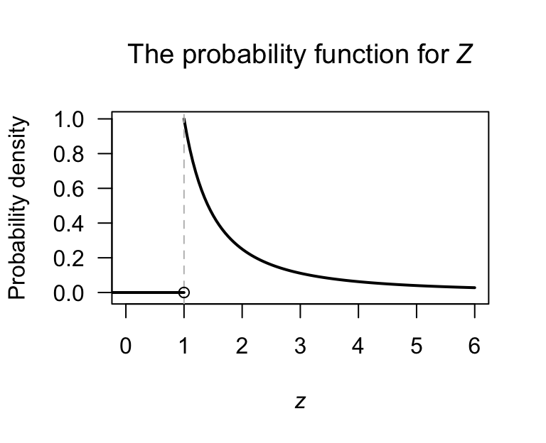
FIGURE 3.1: The probability function for the random variable $Z$. The mean is not defined.

3.2 Expectation of a function of a random variable

While the mean can be expressed in terms of mathematical expectation, mathematical expectation is a more general concept.

Let $X$ be a discrete random variable with a probability function $p_X(x)$, or a continuous random variable with pdf $f_X(x)$. Also assume $g(X)$ is a real-valued function of $X$. We can then define the expected value of $g(X)$.

Definition 3.2 (Expectation for function of a random variable) The expected value of some function $g(\cdot)$ of a random variable $X$ is:

• $\displaystyle\text{E}\big(g(X)\big) = \sum_{x\in R_X} g(x) p_X(x)$ for a discrete random variable $X$ with pmf $p_X(x)$;

• $\displaystyle\text{E}\big(g(X)\big) = \int_{-\infty}^\infty g(x) f_X(x)\,dx$ for a continuous random variable $X$ with pdf $f_X(x)$.

If $Y = g(X)$, write $\mu_Y = \text{E}(Y) = \text{E}\big(g(X)\big)$. Importantly, the expectation operator is a linear operator, as stated below.

Theorem 3.1 (Expectation properties) For any random variable $X$ and constants $a$ and $b$, $$\text{E}(aX + b) = a\text{E}(X) + b.$$

Proof. Assume $X$ is a discrete random variable with probability function $p_X(x)$. By Def. 3.2 with $g(X) = aX + b$, $$\text{E}(aX + b) = \sum_x (ax + b) p_X(x) = a\sum_x p_X(x) + \sum_x b p_X(x) = a\text{E}(X) + b,$$ using that $\sum_x p_X(x) = 1$. (The proof in the continuous case uses the probability function with a pdf, and replaces summations with integrals.)

Example 3.5 (Expectation of a function of a random variable) Consider the random variable $Y = 2x$ where $X$ is defined in Example 3.2. Using Theorem 3.1 with $a = 2$ and $b = 0$, the value of $\text{E}(Y)$ is $$\text{E}(2X) = 2\text{E}(X) = 2 \times 13/6 = 13/3.$$

3.3 Measures of location

Having introduced the idea of mathematical expectation, other descriptions of a random variable can now be introduced.

Two general features of a distribution are the location or centre, and the variability. We have already met the mean (or expected value) as one measure of location.

3.3.1 The mean

The most important measure of location is the mean $\mu = \text{E}(X)$, which has already been defined (Sect. 3.1). The mean is the balance point of the distribution: the expected mean deviation of the random variable from $\mu$ is zero. In other words, $\text{E}(X - \mu) = 0$.

While the mean is commonly used, it is not always a suitable measure of centre: the balance point can be unduly affected by outliers and extreme skewness. We have also seen a situation where the mean is undefined (Example 3.4).

3.3.2 The mode and median

Other measures of centre sometimes may be more appropriate. The mode and median are two common alternatives. The mean, when it is defined, is more useful in theoretical work due to nicer mathematical properties,

Definition 3.3 (Mode) The mode(s) is a value(s) $x\in R_X$ such that:

• $p_X(x)$ attains its maximum (for the discrete case); or
• the value(s) of $x$ at which $f_X(x)$ attains its maximum (for the continuous case).

The mode is not necessarily unique.

Definition 3.4 (Median) The median of a random variable $X$ (or of a distribution) is a number $\nu$ such that
$$\begin{equation} \Pr(X\leq \nu )\geq \frac{1}{2}\text{ and }\Pr(X \geq \nu )\geq \frac{1}{2}. \end{equation}$$

For $X$ discrete, the median is not necessarily unique.

Example 3.6 (Mode and median for discrete distributions) If $X$ is a discrete random variable with probability function defined in Table 3.1 (and shown in Fig. 3.2), the distribution is bimodal (i.e., has two modes), with modes at $x = 3$ and $x = 4$.

The median, say $\nu$, is any value of $X$ in the range $3 < x < 4$, since any number in this range satisfies $\Pr(X \le x) = 0.5$ and $\Pr(X \ge x) = 0.5$. The median is not unique.

TABLE 3.1: A probability distribution

$x$	0	1	2	3	4	5	6	7
$\Pr(X = x)$	$\frac{1}{128}$	$\frac{7}{128}$	$\frac{21}{128}$	$\frac{35}{128}$	$\frac{35}{128}$	$\frac{21}{128}$	$\frac{7}{128}$	$\frac{1}{128}$

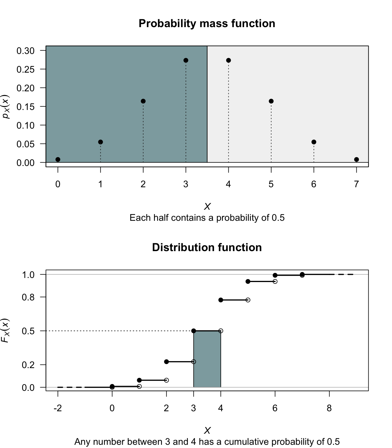
FIGURE 3.2: Finding the median, when it is not unique

Example 3.7 (Expectation for discrete variables) Let $X$ be a discrete random variable with the probability function shown in Table 3.2 (and Fig. 3.3). The mode of this distribution is at $x = 3$. The median is $\nu = 3$ since this is the only value of $X$ that will satisfy Def. 3.4.

TABLE 3.2: A probability distribution

$x$	0	1	2	3	4	5	6
$\Pr(X = x)$	$\frac{1}{64}$	$\frac{6}{64}$	$\frac{15}{64}$	$\frac{20}{64}$	$\frac{15}{64}$	$\frac{6}{64}$	$\frac{1}{64}$

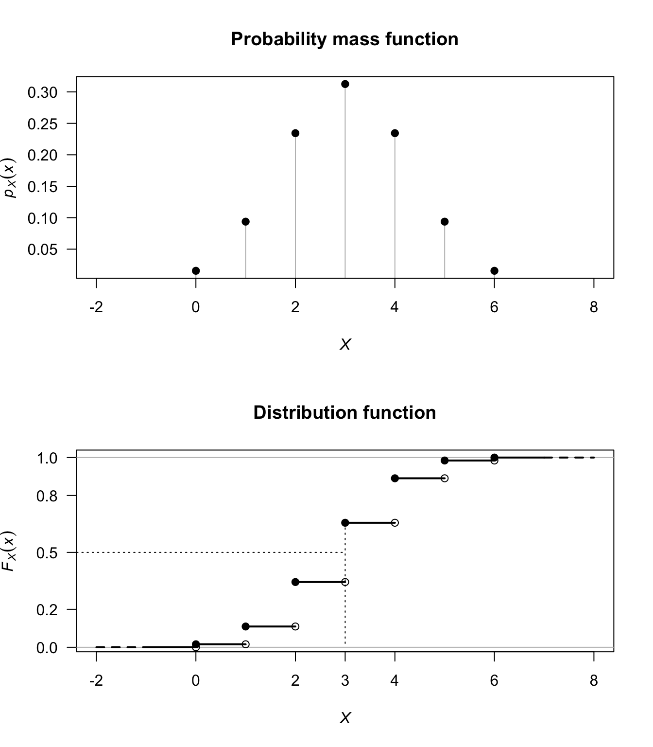
FIGURE 3.3: The probability function and distribution function for $H$

3.4 Measures of variability

Apart from the mean, the most important description of a random variable is the variability: quantifying how the values of the random variable are dispersed. The most important measure of variability is the variance.

3.4.1 The variance and standard deviation

The variance can be expressed as a function of a random variable. (More correctly, we should say “the variance of the distribution of the random variable”, but our language is very common.)

The variance is a measure of the variability of a random variable. A small variance means the observations are nearly the same (i.e., small variation); a large variance means they are quite different.

Definition 3.5 (Variance) The variance of a random variable $X$ (or of the distribution of $X$) is $$\text{var}(X) = \text{E}\big((X - \mu)^2\big)$$ where $\mu = \text{E}(X)$. The variance of $X$ is commonly denoted by $\sigma^2$, or $\sigma^2_X$ if distinguishing among variables is needed.

The variance is the expected value of the squared distance of the values of the random variable from the mean, weighted by the probability function. The unit of measurement for variance is the original unit of measurement squared. That is, if $X$ is measured in metres, the variance of $X$ is in $\text{metres}^2$.

Describing the variability in terms of the original units is more natural, by taking the square root of the variance.

Definition 3.6 (Standard deviation) The standard deviation of a random variable $X$ is defined as the positive square root of the variance (denoted by $\sigma$); i.e., $$\text{sd}(X) = \sigma = +\sqrt{\text{var}(X)}$$

The variance is less popular than the standard deviation in practice to describe variability. In theoretical work, however, the variance is easier to work with than standard deviation (due to the square root), and the variance, rather than standard deviation, features in many results in theoretical statistics.

Example 3.8 (Variance for a die toss) Suppose a fair die is tossed, and $X$ denotes the number of points showing. Then $\Pr(X = x) = 1/6$ for $x = 1, 2, 3, 4, 5, 6$ and $$\mu = \text{E}(X) = \sum_S x\Pr(X = x) = (1 + 2 + 3 + 4 + 5 + 6 )/6 = 7/2.$$ The variance of $X$ is then
$$\begin{align*} \sigma^2 &= \text{var}(X) = \sum (X - \mu)^2 \Pr(X = x)\\ &= \frac{1}{6}\left[ \left(1 - \frac{7}{2}\right)^2 + \left(2 - \frac{7}{2}\right)^2 + \dots + \left(6 - \frac{7}{2}\right)^2 \right] = \frac{70}{24}. \end{align*}$$ The standard deviation is then $\sigma = \sqrt{70/24} = 1.71$.

An important result is known as the computational formula for variance.

Theorem 3.2 (Computational formula for variance) For any random variable $X$, $$\text{var}(X) = \text{E}(X^2) - [\text{E}(X)]^2.$$

Proof. Let $\text{E}(X) = \mu$, then (using the properties of expectation in Theorem 3.1):
$$\begin{align*} \text{var}(X) = \text{E}\left((X - \mu)^2\right) &= \text{E}( X^2 - 2X\mu + \mu^2) \\ &= \text{E}(X^2) - \text{E}(2X\mu) + \text{E}(\mu^2)\\ &= \text{E}(X^2) - 2\mu\text{E}(X) + \mu^2\\ &= \text{E}(X^2) - 2\mu^2 + \mu^2 \\ &= \text{E}(X^2) - \mu^2 \\ &= \text{E}(X^2) - \big(\text{E}(X)\big)^2. \end{align*}$$

This formula is often easier to use to compute $\text{var}(X)$ than using the definition directly.

Example 3.9 (Variance for a die toss) Consider Example 3.9 again. Then
$$\begin{align*} \text{E}(X^2) = \sum_S x^2 \Pr(X = x) &= \frac{1}{6}[1^2 + 2^2 + 3^2 + 4^2 = 5^2 + 6^2]\\ &= 91/6, \end{align*}$$ and so $\text{var}(X) = 91/6 - (7/2)^2 = 70/24$, as before.

Example 3.10 (Variance using computational formula) Consider the continuous random variable $X$ with pdf $$f_X(x) = \begin{cases} 3x(2 - x)/4 & \text{for $0 < x < 2$};\\ 0 & \text{elsewhere}. \end{cases}$$ The variance of $X$ can be computed in two ways: using $\text{var}(X) = \text{E}((X - \mu)^2)$ or using the computational formula. The expected value of $X$ is $$\text{E}(X) = \int_0^2 x.3x(2 - x)4\, dx = 1.$$ To use the computational formula, $$\text{E}(X^2) = \frac{6}{5},$$ and so $\text{var}(X) = \text{E}(X^2) - \big(\text{E}(X)\big)^2 = 1/5$.

Using the definition,
$$\begin{align*} \text{var}(X) = \text{E}\big((X - \text{E}(X))^2\big) &= \text{E}\big((X - 1)^2\big)\\ &= \int_0^2 (x - 1)^2 3x(2 - x)/4\,dx = 1/5. \end{align*}$$

Both methods give the same answer of course, and both methods require initial computation of $\text{E}(X)$. The computational formula requires less work.

The variance represents the expected value of the squared distance of the values of the random variable from the mean. The variance is never negative, and is only zero when all the values of the random variable are identical (that is, there is no variation).

If most of the probability lies near the mean, the dispersion will be small; if the probability is spread out over a considerable range the dispersion will be large.

Example 3.11 (Infinite variance) In Example 3.4, $\text{E}(X)$ was not defined. For that reason, the variance is also undefined, since computing the variance relies on having a finite value for $\text{E}(X)$.

Theorem 3.3 (Variance properties) For any random variable $X$ and constants $a$ and $b$, $$\text{var}(aX + b) = a^2\text{var}(X).$$

Proof. Using the computational formula for the variance:
$$\begin{align*} \text{var}(aX + b) &= \text{E}[ (aX + b)^2 ] - \left[\text{E}(aX + b) \right] ^2\\ &= \text{E}[a^2 X + 2abX + b^2] + (a\mu+b)^2\\ &= a^2 \text{E}[X^2] - a^2\mu^2\\ &= a^2 \text{var}(X). \end{align*}$$

The special case $a = 0$ is instructive: $\text{var}(b) = 0$ when $b$ is constant; that is, a constant has zero variation.

Example 3.12 (Variance of a function of a random variable) Consider the random variable $Y = 4 - 2X$ where $\text{E}(X) = 1$ and $\text{var}(X) = 3$. Then:
$$\begin{align*} \text{E}(Y) &= \text{E}(4 - 2X) = 4 - 2\times\text{E}(X) = 2;\\ \text{var}(Y) &= \text{var}(4 - 2X) = (-2)^2\text{var}(X) = 12. \end{align*}$$

3.4.2 The mean absolute deviation

We have already seen variance and standard deviation are suitable measures of dispersion. Another alternative is the following.

Definition 3.7 (Mean absolute deviation) The mean absolute deviation (MAD) is defined as:

• $\displaystyle \text{E}(|X - \mu|) = \sum_x |x - \mu| p_X(x)$ for a discrete random variable $X$;
• $\displaystyle \text{E}(|X - \mu|) = \int_{-\infty}^\infty |x - \mu| f_X(x)\,dx$ for a continuous random variable $X$.

Example 3.13 (MAD of die toss) Consider the fair die described in Example 3.8. Then $\mu = \text{E}(X) = 7/2$ and thus the MAD of $X$ is
$$\begin{align*} \text{E}(|X - \mu|) &= \sum |x - \mu| \Pr(X = x)\\ &= \frac{1}{6}\left[ \left|1 - \frac{7}{2}\right| +\left|2 - \frac{7}{2}\right| + \dots + \left|6 - \frac{7}{2}\right|\right]\\ &= 1.5. \end{align*}$$

Like the median, the MAD is difficult to use in theoretical work (due to the absolute value). The most-used measure of dispersion is the variance (or standard deviation).

3.5 Higher moments

The idea of a mean and variance are generalised in the following definitions.

Definition 3.8 (Raw moments) The $r$th moment about the origin, or $r$th raw moment, of a random variable $X$ (where $r$ is a positive integer) is defined as:

• $\displaystyle\mu'_r = \text{E}(X^r) = \sum_X x^r p_X(x)$ for the discrete case;
• $\displaystyle\mu'_r = \text{E}(X^r) = \int_{-\infty}^\infty x^r f_X(x)$ for the continuous case.

Definition 3.9 (Central moments) The $r$th central moment, or $r$th moment about the mean (where $r$ is a positive integer), is defined as

• $\displaystyle\mu_r = \text{E}((X - \mu)^r) = \sum_x (x - \mu)^r p_X(x)$ in the discrete case;
• $\displaystyle\mu_r = \text{E}\big((X - \mu)^r\big) = \int_{-\infty}^{\infty} (x - \mu)^r f_X(x)$ in the continuous case.

From these definitions:

• the mean $\mu'_1 = \mu$ is the first moment about the origin, or the first raw moment;
• $\mu'_2 = \text{E}(X^2)$ is the second moment about the origin, or the second raw moment; and
• the variance $\mu_2 = \sigma^2$ is the second moment about the mean or the second central moment.

Higher moments also exist that describe other features of a random variable. One important higher moment is related to skewness.

Definition 3.10 (Skewness) The skewness of a distribution is defined as
$$\begin{equation} \gamma_1 = \frac{\mu_3}{\mu_2^{3/2}}. \tag{3.1} \end{equation}$$

If $\gamma_1 >0$ we say the distribution is positively (or right) skewed, and it is ‘stretched’ in the positive (negative) direction. Similarly, if $\gamma_1 <0$ we say the distribution is negatively (or left) skewed.

Definition 3.11 (Symmetry) The distribution of $X$ is said to be symmetric if, for all $x\in R_X$,

• $\Pr(X = \mu + x) = \Pr(X = \mu - x)$ for the discrete case;
• $\Pr(X = \mu + x) = f_X(\mu - x)$ for the continuous case.

For a symmetric distribution, the mean is also a median of the distribution, as these results show.

For a symmetric distribution, the odd central moments are zero (Exercise 3.10). This suggests that odd central moments can be used to measure the asymmetry of a distribution (as in Def. 3.10).

Example 3.14 (Skewness) Consider the random variable $X$ in Example 3.10, where $f_X(x) = x(2 - x)$ for $0 < x < 2$. In that example, we found $\text{E}(X) = \mu'_1 = 1$ and $\text{E}(X^2) = \mu_2 = 6/5$. Then, $$\mu_3 = \int_0^2 (x - 1)^3 3x(2 - x)/4 \,dx = 0,$$ so that the skewness in Eq. (3.1) will be zero. This is expected, since the distribution is symmetric (Fig. 3.4).

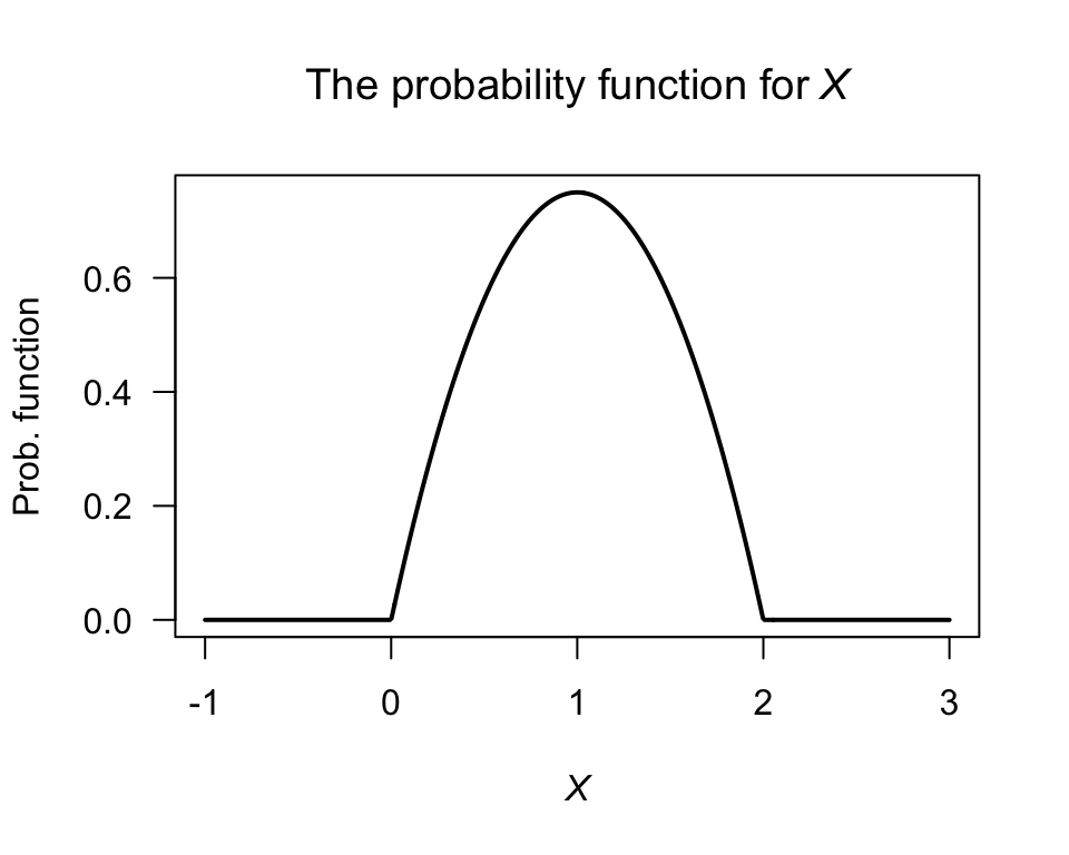
FIGURE 3.4: The probability density function for $X$

Instead of central moments themselves, using expressions unaffected by a linear transformation of the type $Y = aX + b$ (for constants $a$ and $b$) are convenient. The ratio $(\mu_r)^p / (\mu_p)^r$ is such an expression, and the simplest form is a function of $\mu^2_3/\mu_2^3$.

Example 3.15 (Skewness) Consider the random variable $Y$ with pmf $$p_Y(y) = \begin{cases} 0.2 & \text{for $y = 5$};\\ 0.3 & \text{for $y = 6$};\\ 0.5 & \text{for $y = 7$};\\ 0 & \text{elsewhere}. \end{cases}$$ Then $\mu'_1 = \text{E}(Y) = (5\times 0.2) + (6\times 0.3) + (7\times 0.5) = 6.3$. Likewise, $\mu_2 = \text{E}\big((y - 6.3)^2 p_Y(y) \big) = 0.1982$ and $\mu_3 = \text{E}\big((y - 6.3)^3 p_Y(y) \big) = 0.02457$. Hence, the skewness is $$\gamma_1 = \frac{\mu_3}{\mu_2^{3/2}} = \frac{0.02457}{0.1982^{3/2}} = 0.02785,$$ so the distribution has positive skewness.

Another ratio gives a measure of kurtosis, which measures the heaviness of the tails in a distribution.

Definition 3.12 (Kurtosis) The kurtosis of a distribution is defined as
$$\begin{equation*} \frac{\mu_4}{\mu^2_2}. \end{equation*}$$ The excess kurtosis of a distribution is defined as
$$\begin{equation*} \gamma_2 = \frac{\mu_4}{\mu^2_2} - 3. \end{equation*}$$

Excess kurtosis is commonly used, and sometimes is just called ‘kurtosis’.

Large values of kurtosis corresponds to greater proportion of the distribution in the tails. The excess kurtosis is defined so that the normal, or bell-shaped, distribution (Sect. 5.3), which has a kurtosis of 3, has a excess kurtosis of zero. Then:

• distributions with negative excess kurtosis are called platykurtic. These distribution have fewer, or less extreme, observations in the tail compared to the normal distribution (‘thinner tails’). Examples include the Bernoulli distribution.
• distributions with positive excess kurtosis are called leptokurtic. These distribution have more, or more extreme, observations in the tail compared to the normal distribution (‘fatter tails’). Examples include the exponential and Poisson distributions.
• distributions with zero excess kurtosis are called mesokurtic. The normal distribution is the obvious example.

Example 3.16 (Uses of skewness and kurtosis) Monypenny and Middleton (1998b) and Monypenny and Middleton (1998a) use the skewness and kurtosis to analyse wind gusts at Sydney airport.

Example 3.17 (Uses of skewness and kurtosis) Galagedera, Henry, and Silvapulle (2002) used higher moments in a capital analysis pricing model for Australian stock returns.

Example 3.18 (Skewness and kurtosis) Consider the discrete random variable $U$ from Example 3.1. The raw moments are
$$\begin{align*} \mu'_r = \text{E}(U^r) &= \sum_{u = -1, 0, 1} u^r \frac{u^2 + 1}{5} \\ &= (-1)^r \frac{ (-1)^2 + 1}{5} + (0)^r \frac{ (0)^2 + 1}{5} + (1)^r \frac{ (1)^2 + 1}{5} \\ &= \frac{2(-1)^r}{5} + 0 + \frac{2}{5} \\ &= \frac{2}{5}[ (-1)^r + 1] \end{align*}$$ for the $r$th raw moment. Then,
$$\begin{align*} \text{E}(X) &= \mu'_1 = \frac{2}{5}[ (-1)^1 + 1 ] = 0;\\ \text{E}(X^2) &= \mu'_2 = \frac{2}{5}[ (-1)^2 + 1 ] = 4/5;\\ \text{E}(X^3) &= \mu'_1 = \frac{2}{5}[ (-1)^3 + 1 ] = 0;\\ \text{E}(X^4) &= \mu'_2 = \frac{2}{5}[ (-1)^4 + 1 ] = 4/5. \end{align*}$$ Since $\text{E}(U) = 0$, then the $r$th central and raw moments are the same: $\mu'_r = \mu_r$. Notice that once the initial computations to find $\mu'_r$ are complete, the evaluation of any raw moment is simple.

The skewness is $$\gamma_1 = \frac{\mu_3}{\mu_2^{3/2}} = \frac{0}{(4/5)^{3/2}} = 0,$$ so the distribution is symmetric. The excess kurtosis is $$\gamma_2 = \frac{\mu_4}{\mu_2^2} -3 = \frac{4/5}{(4/5)^2} -3 = -7/4,$$ so the distribution is platykurtic.

By themselves, the mean, variance, skewness and kurtosis do not completely describe a distribution; many different distributions can be found having a given mean, variance, skewness and kurtosis. However, in general, all the moments of a distribution together define the distribution. This leads to the idea of a moment-generating function.

3.6 Moment-generating functions

3.6.1 Definition

So far, the distribution of a random variable has been described using a probability function or a distribution function. Sometimes, however, working with a different representation is useful (for example, see Sect. 7.4).

In this section, the moment-generating function is used to represent the distribution of the probabilities of a random variable. As the name suggests, this function can be used to generate any moment of a distribution. Other uses of the moment-generating function are seen later (see Sect. 7.4).

Definition 3.13 (Moment-generating function (mgf)) The moment-generating function (or mgf) $M_X(t)$ of the random variable $X$ is defined as:

• $\displaystyle M_X(t) = \text{E}\big(\exp(tX)\big) = \sum_x \exp(tx) p_X(x)$ in the discrete case;
• $\displaystyle M_X(t) = \text{E}\big(\exp(tX)\big) = \int_{-\infty}^\infty \exp(tx) f_X(x)$ in the continuous case.

The mgf is defined as an infinite series or an infinite integral. Such an expression may not always exist (that is, converge to a finite value) for all values of $t$, so the mgf may not be defined for all values of $t$. Note that the mgf always exists for $t = 0$; in fact $M_X(0) = 1$.

Provided the mgf is defined for some values of $t$ other than zero, it uniquely defines a probability distribution, and we can use it to generate the moments of the distribution as described in Theorem 3.4.

Moment-generating functions are related to Laplace transformations.

Example 3.19 (Moment-generating function) Consider the random variable $Y$ with pdf $$f_Y(y) = \begin{cases} \exp(-y) & \text{for $y > 0$};\\ 0 & \text{elsewhere.} \end{cases}$$ The mgf is
$$\begin{align*} M_Y(t) = \text{E}[\exp(tY)] &= \int_0^\infty \exp(ty)\exp(-y)\, dy \\ &= \int_0^\infty \exp\{ y(t-1) \}\, dy \\ &= \left.\frac{1}{t-1} \exp\{y(t-1)\}\right|_{y = 0}^{y = \infty}\\ &= (1 - t)^{-1} \end{align*}$$ provided $t - 1 < 0$; that is, for $t < 1$. If $t > 1$, the integral does not converge. For example, if $t = 2$, $$\left. \frac{1}{2 - 1} \exp(y)\right|_{y = 0}^{y = \infty} = \exp(0) - \lim_{y\to\infty} \exp(y)$$ which does not converge.

Example 3.20 (Mgf for die rolls) Consider the pf of $X$, the outcome of tossing a fair die (Example 3.8). The mgf of $X$ is
$$\begin{align*} M_X(t) &= \text{E}(\exp(tX)) = \sum_{x = 1}^6 \exp(tx) p_X(x)\\ &= \frac{1}{6}\left(e^t + e^{2t} + e^{3t} + e^{4t} + e^{5t} + e^{6t}\right), \end{align*}$$ which exists for all values of $t$.

3.6.2 Using the mgf to generate moments

Replacing $\exp(xt)$ by its series expansion (App. A) in the definition of the mgf gives
$$\begin{align*} M_X(t) & = {\sum_x} \left(1 + xt + \frac{x^2t^2}{2!} + \dots\right) \Pr(X = x)\\ & = 1 + \mu'_1t + \mu'_2 \frac{t^2}{2!} +\mu'_3 \frac{t^3}{3!} + \dots \end{align*}$$ Then, the $r$th moment of a distribution about the origin is seen to be the coefficient of $t^r/r!$ in the series expansion of $M_X(t)$:
$$\begin{align*} \frac{d M_X(t)}{dt} & = \sum_x x\,e^{xt}\Pr(X = x)\\ \frac{d^2 M_X(t)}{dt^2} & = \sum_x x^2\,e^{xt} \Pr(X = x), \end{align*}$$ and so, for each positive integer $r$, $$\frac{d^r M_X(t)}{dt^r} = \sum_x x^re^{xt}\Pr(X = x).$$ On setting $t = 0$, $d M_X(t)/dt\Big|_{t = 0} = \text{E}(X)$, $d^2M_X(t)/dt^2 \Big|_{t = 0} = \text{E}(X^2)$, and for each positive integer $r$,
$$\begin{equation} \frac{d^r M_X(t)}{dt^r}\Big|_{t = 0} = \text{E}(X^r). \end{equation}$$ (Sometimes, $d^r M_X(t)/dt^r\Big|_{t = 0}$ is written as $M^{(r)}(0)$ for brevity.) This result is summarised in the following theorem.

Theorem 3.4 (Moments) The $r$th moment $\mu'_r$ of the distribution of the random variable $X$ about the origin is given by either

1. the coefficient of $t^r/r!, r = 1, 2, 3,\dots$ in the power series expansion of $M_X(t)$; or
2. $\displaystyle \mu'_r = \left.\frac{d^rM(t)}{dt^r}\right|_{t = 0}$ where $M_X(t)$ is the mgf of $X$.

Example 3.21 (Mean and variance from a MF) Continuing Example 3.19, the mean and variance of $Y$ can be found from the mgf. To find the mean, first find $$\frac{d}{dt}M_Y(t) = (1 - t)^{-2}.$$ Setting $t = 0$ gives the mean as $\text{E}(Y) = 1$. Likewise, $$\frac{d^2}{dt^2}M_Y(t) = 2(1 - t)^{-3}.$$ Setting $t = 0$ gives $\text{E}(Y^2) = 2$. The variance is therefore $\text{var}[Y] = 2 - 1^2 = 1$.

Once the moment-generating function has been computed, raw moments can be computed using $$\text{E}(Y^r) = \mu'_r = \left.\frac{d^r}{dt^r} M_Y(t)\right|_{t = 0}.$$

3.6.3 Some useful results

The moment-generating function can be used to derive the distribution of a function of a random variable (see Sect. 7.4). The following theorems are valuable for this task.

Theorem 3.5 (Mgf of linear combinations) If the random variable $X$ has mgf $M_X(t)$ and $Y = aX + b$ where $a$ and $b$ are constants, then the mgf of $Y$ is $$M_Y(t) = \text{E}\big(\exp\{t(aX + b)\}\big) = \exp(bt) M_X(at).$$

Theorem 3.6 (Mgf of independent rvs) If $X_1$, $X_2$, $\dots$, $X_n$ are $n$ independent random variables, where $X_i$ has mgf $M_{X_i}(t)$, then the mgf of $Y = X_1 + X_2 + \cdots X_n$ is $$M_Y(t) = \prod_{i = 1}^n M_{X_i}(t).$$

Proof. The proofs are left as an exercise.

Note that in the special case when all the random variables are independently and identically distributed in Theorem 3.5, we have $$M_Y(t) = [M_{X_i}(t)]^n.$$

Example 3.22 (Mgf of linear combinations) Consider the random variable $X$ with pf $$p_X(x) = 2(1/3)^x \qquad \text{for $x = 1, 2, 3, \dots$}$$ and zero elsewhere. The mgf of $X$ is
$$\begin{align*} M_X(t) &= \sum_{x: p(x)>0} \exp(tx) p_X(x) \\ &= \sum_{x = 1}^\infty \exp(tx) 2(1/3)^x \\ &= 2\sum_{x = 1}^\infty (\exp(t)/3)^x \\ &= 2\left\{ \frac{\exp(t)}{3} + \left(\frac{\exp(t)}{3}\right)^2 + \left(\frac{\exp(t)}{3}\right)^3 + \dots\right\} \\ &= \frac{2\exp(t)}{3 - \exp(t)} \end{align*}$$ where $\sum_{y = 1}^\infty a^y = a/(1 - a)$ for $a < 1$ has been used (App. A); here $a = \exp(t)/3$.

Next consider finding the mgf of $Y = (X - 2)/3$. From Theorem 3.5 with $a = 1/3$ and $b = -2/3$, $$M_Y(t) = \exp(-2t/3) M_X(t/3) = \frac{2\exp\{(-t)/3\}}{3 - \exp(t/3)}.$$ In practice, rather than identify $a$ and $b$ and remember Theorem 3.5, problems like this are best solved directly from the definition of the mgf:
$$\begin{align*} M_Y(t) = \text{E}(\exp(tY)) &= \text{E}(\exp\{t(X - 2)/3\})\\ &= \text{E}(\exp\{tX/3 - 2t/3\})\\ &= \exp(-2t/3) M_X(t/3) \\ &= \frac{2\exp\{(-t)/3\}}{3 - \exp(t/3)}. \end{align*}$$

3.6.4 Determining the distribution from the mgf

The mgf (if it exists) completely determines the distribution of a random variable hence, given a mgf, deducing the probability function should be possible. For some distributions, the pdf cannot be written in closed form (so the pdf can only be evaluated numerically), but the mgf is relatively simple to write down.

In the discrete case, the mgf is defined as
$$\begin{equation} M_X(t) = \text{E}(\exp(tX)) = \sum_X e^{tx} p_X(x) \tag{3.2} \end{equation}$$ for $X$ discrete with pf $p_X(x)$. This can be expressed as
$$\begin{align*} M_X(t) &= \exp(t x_1) p_X(x_1) + \exp(t x_2)p_X(x_2) + \dots\\ &= \exp(t x_1) \Pr(X = x_1) + \exp(t x_2)\Pr(X = x_2) + \dots\\ \end{align*}$$ and so the probability function of $Y$ can be deduced from the mgf.

Example 3.23 (Distribution from the mgf) Suppose a discrete random variable $D$ has the mgf $$M_D(t) = \frac{1}{3} \exp(2t) + \frac{1}{6}\exp(3t) + \frac{1}{12}\exp(6t) + \frac{5}{12}\exp(7t).$$ Then, by the definition of the mgf in the discrete case given above, the coefficient of $t$ in the exponential indicates values of $D$, and the coefficient indicates the probability of that value of $y$:
$$\begin{align*} M_D(t) &= \overbrace{\frac{1}{3} \exp(2t)}^{D = 2} + \overbrace{\frac{1}{6}\exp(3t)}^{D = 3} + \overbrace{\frac{1}{12}\exp(6t)}^{D = 6} + \overbrace{\frac{5}{12}\exp(7t)}^{D = 7}\\ &= \Pr(D = 2)\exp(2t) + \Pr(D = 3)\exp(3t) + \\ & \quad \Pr(D = 6)\exp(6t) + \Pr(D = 7)\exp(7t). \end{align*}$$ So the pf is $$p_D(d) = \begin{cases} 1/3 & \text{for $d=2$}\\ 1/6 & \text{for $d=3$}\\ 1/12 & \text{for $d=6$}\\ 5/12 & \text{for $d=7$}\\ 0 & \text{otherwise} \end{cases}$$ (Of course, it is easy to check by computing the mgf for $D$ from the pf found above; you should get the original mgf.)

Sometimes, using the results in App. A can be helpful.

Example 3.24 (Distribution from the mgf) Consider the mgf $$M_X(t) = \frac{\exp(t)}{3 - 2\exp(t)}.$$ To find the corresponding probability function, one approach is to write the mgf as $$M_X(t) = \frac{\exp(t)/3}{1 - 2\exp(t)/3}.$$ This is the sum of a geometric series (Eq. (A.5)): $$a + ar + ar^2 + \ldots + ar^{n - 1} \rightarrow \frac{a}{1 - r} \text{ as $n \rightarrow \infty$},$$ where $a = \exp(t)/3$ and $r = 2\exp(t)/3$. Hence the mgf can be expressed as $$\frac{1}{3}\exp(t) + \frac{1}{3}\left(\frac{2}{3}\right) \exp(2t) + \frac{1}{3}\left(\frac{2}{3}\right)^2 \exp(3t) + \dots$$ so that the probability function can be deduced as
$$\begin{align*} \Pr(X = 1) &= \frac{1}{3};\\ \Pr(X = 2) &= \frac{1}{3}\left(\frac{2}{3}\right);\\ \Pr(X = 3) &= \frac{1}{3}\left(\frac{2}{3}\right)^2, \end{align*}$$ or, in general, $$p_x(x) = \frac{1}{3}\left( \frac{2}{3}\right)^{x - 1}\quad\text{for $x = 1, 2, 3, \dots$}.$$ (Later, this will be identified as a geometric distribution.)

The case of a continuous random variable is more involved. Suppose the continuous random variable $X$ has the mgf $M_X(t)$. Then the probability density function is (see Abramowitz and Stegun (1964), 26.1.10)
$$\begin{equation} f_X(x) = \frac{1}{2\pi} \int_{-\infty}^{\infty} M_X(it) \exp(-itx)\, dt, \tag{3.3} \end{equation}$$ where $i = \sqrt{-1}$.

Example 3.25 (Distribution from the mgf) Consider the mgf for a continuous random variable $X$ such that $M_X(t) = \exp(t^2/2)$, for $y\in\mathbb{R}$ and $t\in\mathbb{R}$. Then, $M_X(it) = \exp\left( (it)^2/2 \right) = \exp(-t^2/2)$. Using Eq. (3.3), the pdf is:
$$\begin{align*} f_X(x) &= \frac{1}{2\pi} \int_{-\infty}^{\infty} \exp(-t^2/2) \exp(-itx)\, dt,\\ &= \frac{1}{2\pi} \int_{-\infty}^{\infty} \exp(-t^2/2)\left[ \cos(-tx) + i\sin(-itx)\right]\, dt, \end{align*}$$ since $x\in\mathbb{R}$ and $t\in\mathbb{R}$. Extracting just the real components:
$$\begin{align*} f_X(x) &= \frac{1}{2\pi} \int_{-\infty}^{\infty} \exp(-t^2/2) \cos(-tx) \, dt\\ &= \frac{1}{2\pi} \left( \sqrt{2\pi} \exp( -x^2/2 ) \right) = \frac{1}{ \sqrt{2\pi} } \exp( -x^2/2 ), \end{align*}$$ which will later be identified as a normal distribution with a mean of zero, and standard deviation of one.

In practice, using Eq. (3.3) can become tedious or intractable for producing a closed form expression for the pdf. However, Eq. (3.3) has been used to compute numerical values of the probability density function. For example, Dunn and Smyth (2008) used Eq. (3.3) to evaluate the Tweedie distributions (Dunn and Smyth 2001), for which (in general) the pdf has no closed form, but does have a simple mgf.

3.7 Tchebysheff’s inequality

Tchebysheff’s inequality applies to any probability distribution, and is sometimes useful in theoretical work or to provide bounds on probabilities.

Theorem 3.7 (Tchebysheff's theorem) Let $X$ be a random variable with finite mean $\mu$ and variance $\sigma^2$. Then for any positive $k$,
$$\begin{equation} \Pr\big(|X - \mu| \geq k\sigma \big)\leq \frac{1}{k^2} \tag{3.4} \end{equation}$$ or, equivalently
$$\begin{equation} \Pr\big(|X - \mu| < k\sigma \big)\geq 1 - \frac{1}{k^2}. \end{equation}$$

Proof. The proof for the continuous case only is given. Let $X$ be continuous with pdf $f(x)$. For some $c > 0$, then
$$\begin{align*} \sigma^2 & = \int^\infty_{-\infty} (x - \mu )^2f(x)\,dx\\ & = \int^{\mu -\sqrt{c}}_{-\infty} (x - \mu )^2f(x)\, dx + \int^{\mu + \sqrt{c}}_{\mu-\sqrt{c}}(x - \mu )^2f(x)\,dx + \int^\infty_{\mu + \sqrt{c}}(x - \mu)^2f(x)\,dx\\ & \geq \int^{\mu -\sqrt{c}}_{-\infty} (x - \mu )^2f(x)\,dx + \int^\infty_{\mu + \sqrt{c}}(x - \mu )^2f(x)\,dx, \end{align*}$$ since the second integral is non-negative. Now $(x - \mu )^2 \geq c$ if $x \leq \mu -\sqrt{c}$ or $x\geq \mu + \sqrt{c}$. So in both the remaining integrals above, replace $(x - \mu )^2$ by $c$ without altering the direction of the inequality:
$$\begin{align*} \sigma^2 &\geq c \int^{\mu -\sqrt{c}}_{-\infty} f(x)\,dx + c\int^\infty_{\mu + \sqrt{c}}f(x)\,dx\\ &= c\,\Pr(X \leq \mu - \sqrt{c}\,) + c\,\Pr(X \geq \mu + \sqrt{c}\,)\\ &= c\,\Pr(|X - \mu| \geq \sqrt{c}\,). \end{align*}$$ Putting $\sqrt{c} = k\sigma$, Eq. (3.4) is obtained.

With the probability function or pdf of a random variable $X$, then $\text{E}(X)$ and $\text{var}(X)$ can be found, but the converse is not true. That is, from a knowledge of $\text{E}(X)$ and $\text{var}(X)$ we cannot reconstruct the probability distribution of $X$ and hence cannot compute probabilities such as $\Pr(|X - \mu| \geq k\sigma)$. Nonetheless, using Tchebysheff’s inequality we can find a useful bound to either the probability outside or inside of $\mu \pm k\sigma$.

3.8 Exercises

Selected answers appear in Sect. D.3.

Exercise 3.1 The pdf for the random variable $Y$ is defined as $$f_Y(y) = \begin{cases} 2y + k & \text{for $1\le y \le 2$};\\ 0 & \text{elsewhere}. \end{cases}$$

1. Find the value of $k$.
2. Plot the pdf of $Y$.
3. Compute $\text{E}(Y)$.
4. Compute $\text{var}(Y)$.
5. Compute $\Pr(Y > 1.5)$.

Exercise 3.2 The pmf for the random variable $D$ is defined as $$p_D(d) = \begin{cases} 1/2 & \text{for $d = 1$};\\ 1/4 & \text{for $d = 2$};\\ k & \text{for $d = 3$};\\ 0 & \text{otherwise}, \end{cases}$$ for a constant $k$.

1. Compute the mean and variance of $D$.
2. Find the mgf for $D$.
3. Compute the mean and variance of $D$ from the mgf.
4. Compute $\Pr(D < 3)$.

Exercise 3.3 (This Exercise follows Ex. 2.9.) Five people, including you and a friend, line up at random. The random variable $X$ denotes the number of people between yourself and your friend.

Use the probability function of $X$ found in Ex. 2.9, and find the mean number of people between you and your friend. Simulate this in R to confirm your answer.

Exercise 3.4 The mgf of the discrete random variable $Z$ is $$M_Z(t) = [0.3\exp(t) + 0.7]^2.$$

1. Compute the mean and variance of $Z$.
2. Find the pf of $Z$.

Exercise 3.5 The mgf of $G$ is $M_G(t) = (1 - \beta t)^{-\alpha}$ (where $\alpha$ and $\beta$ are constants). Find the mean and variance of $G$.

Exercise 3.6 Suppose that the pdf of $X$ is $$f_X(x) = \begin{cases} 2(1 - x) & \text{for $0 < x < 1$};\\ 0 & \text{otherwise}. \end{cases}$$

1. Find the $r$th raw moment of $X$.
2. Find $\text{E}\big[(X + 3)^2\big]$ using the previous answer.
3. Find the variance of $X$.

Exercise 3.7 Consider the pdf $$f_Y(y) = \frac{2}{y^2}\qquad y\ge 2.$$

1. Show that the mean of the distribution is not defined.
2. Show that the variance does not exist.
3. Plot the probability density function over a suitable range.
4. Plot the distribution function over a suitable range.
5. Determine the median of the distribution.
6. Determine the interquartile range of the distribution.
   (The interquartile range is a measure of spread, and is calculated as the difference between the third quartile and the first quartile. The first quartile is the value below which $25$% of the data lie; the third quartile is the value below which $75$% of the data lie.)
7. Find $\Pr(Y > 4 \mid Y > 3)$.

Exercise 3.8 The Cauchy distribution has the pdf
$$\begin{equation} f = \frac{1}{\pi(1 + x^2)}\quad\text{for $x\in\mathbb{R}$}. \tag{3.5} \end{equation}$$

1. Use R to draw the probability density function.
2. Compute the distribution function for $X$. Again, use R to draw the function.
3. Show that the mean of the Cauchy distribution is not defined.
4. Find the variance and the mode of the Cauchy distribution.

Exercise 3.9 The exponential distribution has the pdf $$f_Y(y) = \frac{1}{\lambda}\exp( -y/\lambda)$$ (for $\lambda > 0$) for $y > 0$ and is zero elsewhere.

1. Determine the moment-generating function of $Y$.
2. Use the moment-generating function to compute the mean and variance of the exponential distribution.

Exercise 3.10 Prove that for a continuous random variable $X$ which has a distribution that is symmetric about 0 then $M_X(t) = M_{-X}(t)$. Hence prove that for such a random variable, all odd moments about the origin are zero.

Exercise 3.11 (This exercise follows from Exercise 2.7.)

In a study modelling waiting times at a hospital (Khadem et al. 2008), patients are classified into one of three categories:

• Red: Critically ill or injured patients.
• Yellow: Moderately ill or injured patients.
• Green: Minimally injured or uninjured patients.

For ‘Yellow’ patients, the service time of doctors are modelled using a triangular distribution, with a minimum at $3.5$ mins, a maximum at $30.5$ minutes and a mode at $5$ mins.

1. Compute the mean of the service times.
2. Compute the variance of the service times.

Exercise 3.12 The characteristic function of a random variable $X$, denoted $\varphi(t)$, is defined as $\varphi_X(t) = \text{E}[\exp(i t X)]$, where $i = \sqrt{-1}$. Unlike the mgf, the characteristic function is always defined, so is sometimes preferred over the mgf.

1. Show that $M_X(t) = \varphi_X(-it)$.
2. Show that the mean of a random variable $X$ is given by $-i\varphi'(0)$ (where, as before, the notation means to compute the derivative of $\varphi(t)$ with respect to $t$, and evaluate at $t = 0$).

Exercise 3.13 You will find Sect. A.2 useful.

1. Write down the first three terms and general term of the expansion of $(1 - a)^{-1}$.
2. Write down the first three terms and general term of the expansion of $\text{E}\left[(1 - tX)^{-1}\right]$.
3. Suppose $R_X(t) = \text{E}\left [(1 - tX)^{-1} \right]$, called the geometric generating function of $X$. Suppose the random variable $Y$ has a uniform distribution on $(0, 1)$; i.e., $f_Y(y) = 1$ for $0 < y < 1$. Determine the geometric generating function of $Y$ from the definition of the expected value. Your answer will involve a term $\log(1 - t)$.
4. Using the answer in Part 3, expand the term $\log(1 - t)$ by writing in terms of the infinite series.
5. Equate the two series expansions in Part 2 and Part 4 to determine an expression for $\text{E}(Y^n)$, $n = 1, 2, 3,\dots$.

Exercise 3.14 Suppose the random variable $X$ is defined as $$f_X(x) = k (3x^2 + 4)\quad\text{for $-c < x < c$},$$ and is zero elsewhere. Solve for $c$ and $k$ if $\text{var}(X) = 28/15$. (Hint: Make sure you use the properties of the given probability distribution before embarking on complicated expressions!)

Exercise 3.15 Benford’s law (also see Exercise 2.15) describes the distribution of the leading digits of numbers that span many orders of magnitudes (e.g., lengths of rivers) as $$p_D(d) = \log_{10}\left( \frac{d + 1}{d} \right) \quad\text{for $d\in\{1, 2, \dots 9\}$},$$ Find the mean of $D$ (i.e., the mean leading digit).

Exercise 3.16 The von Mises distribution is used to model angular data. The probability function is $$p_Y(y) = k \exp\{ \lambda\cos(y - \mu) \}$$ for $0\le y < 2\pi$, $0 \le \mu < 2\pi$ where $\mu$ is the mean, and with $\lambda > 0$.

1. Show that the constant $k$ is a function of $\lambda$ only.
2. Find the median of the distribution.
3. Using R, numerically integrate to find the value $k$ when $\mu = \pi/2$ and $\lambda = 1$.
4. The distribution function has no closed form. Use R to plot the distribution function for $\mu = \pi/2$ with $\lambda = 1$.

Exercise 3.17 The inverse Gaussian distribution has the pdf $$P_Y(y) = \frac{1}{\sqrt{2\pi y^3\phi}} \exp\left\{ -\frac{1}{2\phi} \frac{(y - \mu)^2}{y\mu^2}\right\}$$ for $y > 0$, $\mu > 0$ and $\phi > 0$.

1. Plot the distribution for $\mu = 1$ for various values of $\phi$; comment.
2. The mgf is $$M_Y(t) = \exp\left\{ \frac{\lambda}{\mu} \left( 1 - \sqrt{1 - \frac{2\mu^2 t}{\lambda}} \right) \right\}.$$ Use the mgf to deduce the mean and variance of the inverse Gaussian distribution.

Exercise 3.18 Consider the random variable $W$ such that $$f_W(w) = \frac{c}{w^3}\quad\text{for $w > c$.}$$

1. Find the value of $c$.
2. Find $\text{E}[W]$.
3. Find $\text{var}[W]$.

Exercise 3.19 The Pareto distribution has the distribution function $$F_X(x) = \begin{cases} 1 - \left(\frac{k}{x}\right)^\alpha & \text{for $x > k$}\\ 0 & \text{elesewhere}, \end{cases}$$ for $\alpha > 0$ and parameter $k$,

1. What values of $k$ are possible?
2. Find the density function for the Pareto distribution.
3. Compute the mean and variance for the Pareto distribution.
4. Find the mode of the Pareto distribution.
5. Plot the distribution for $\alpha = 3$ and $k = 3$.
6. For $\alpha = 3$ and $k = 3$, compute $\Pr(X > 4 \mid X < 5)$.
7. The Pareto distribution is often used to model incomes. For example, the “$80$-–$20$ rule” states that $20$% of people receive $80$% of all income (and, further, that $20$% of the highest-earning $20$% receive $80$% of that $80$%). Find the value of $\alpha$ for which this rule holds.

Exercise 3.20 A mixture distribution is a mixture of two or more univariate distributions. For example, the heights of all adults may follow a mixture distribution: one normal distribution for adult females, and another for adult males. For a set of probability functions $p^{(i)}_X(x)$ for $i = 1, 2, \dots n$ and a set of weights $w_i$ such that $\sum w_i = 1$ and $w_i \ge 0$ for all $i$, the mixture distribution $f_X(x)$ is $$f_X(x) = \sum_{i = 1}^n w_i p^{(i)}_X(x).$$

1. Compute the distribution function for $p_X(x)$.
2. Compute the mean and variance of $f_X(x)$.
3. Consider the case where $p^{(i)}_X(x)$ has a normal distribution for $i = 1, 2, 3$, where the means are $-1$, $2$, and $4$ respectively, and the variances are $1$, $1$ and $4$ respectively. Plot the probability density function of $f_X(x)$ for various instructive values of the weights.
4. Suppose heights of female adults have a normal distribution with mean $163$ cm and a standard deviation of $5$ cm, and adult males have heights with a mean of $175$ cm with standard deviation of $7$ cm, and constitute $48$ % of the population (Australian Bureau of Statistics 1995). Deduce and plot the probability density of heights of adult Australians.

Exercise 3.21 Consider the distribution such that $$p_X(x) = \begin{cases} \frac{1}{K} & \text{for $x = 1$};\\ \frac{1}{x(x - 1)} & \text{for $x = 2, 3, \dots, K$};\\ 0 & \text{elsewhere} \end{cases}$$ for $K > 2$.

1. Find the mean and variance of $X$ (as well as possible).
2. Plot the distribution for various values of $K$.
3. For $K = 6$, determine the mgf.

Exercise 3.22 The random variable $V$ has the pmf $$f_V(v) = (1 - p)^{v - 1} p\quad\text{for $v = 1, 2, \dots$},$$ and zero elsewhere.

1. Show that this is a valid pmf.
2. Find $\text{E}[V]$.
3. Find $\text{var}[V]$.

Exercise 3.23 Two dice are rolled. Deduce the pmf for the absolute difference between the two numbers that appear uppermost.

Exercise 3.24 The random variable $Y$ has the pmf $$p_Y(y) = \frac{e^{-\lambda}\lambda^y}{y!}\quad\text{for $y = 0, 1, 2, \dots$},$$ where $\lambda > 0$. Find the mgf of $Y$, and hence show that $\text{E}(Y) = \text{var}(Y)$.

Exercise 3.25 In practice, some distributions cannot be written in closed form, but can be given by writing their moment-generating function. To evaluate the density then requires an infinite summation or an infinite integral. Given a moment-generating function $M(t)$, the probability density function can be reconstructed numerically from the integral using the inversion formula in Eq. (3.3).

The evaluation of the integral generally requires advanced numerical techniques. In this question, we just consider the exponential distribution as a simple example to demonstrate the use of the inversion formula.

1. Write down the expression in Eq. (3.3) in the case of the exponential distribution, for which $M_X(t) = \lambda/(\lambda - t)$ for $t < \lambda$.
2. Only the real part of the integral is needed. Extract the real parts of this expression, and simplify the integrand. (The integrand is the expression to be integrated.)
3. Plot the integrand from the last part from $t = -50$ to $t = 2$ in the case $\lambda = 2$ and $x = 1$.

Exercise 3.26 The density function for the random variable $X$ is given as $$f(x) = x e^{-x} \quad\text{for $x > 0$}.$$

1. Determine the moment-generating function (mgf) of $X$.
2. Use the mgf to verify that $\text{E}(X) = \text{var}(X)$.
3. Suppose that $Y = 1 - X$. Determine $\text{E}(Y)$.

Exercise 3.27 The Gumbel distribution has the cumulative distribution function
$$\begin{equation} F(x; \mu, \beta) = \exp\left[ -\exp\left( -\frac{x - \mu}{\sigma}\right)\right] \tag{3.6} \end{equation}$$ (for $\mu > 0$ and $\sigma > 0$) and is often used to model extremes values (such as the distribution of the maximum river height).

1. Deduce the probability function for the Gumbel distribution.
2. Plot the Gumbel distribution for a variety of parameters.
3. The maximum daily precipitation (im mm) in Oslo, Norway, is well-modelled using a Gumbel distribution with $\mu = 2.6$ and $\sigma = 1.86$. Draw this distribution, and explain what it means.

Exercise 3.28 The density function for the random variable $X$ is given as $$f(x) = x e^{-x} \quad\text{for $x > 0$}.$$

1. Determine $\text{E}(X)$.
2. Verify that $\text{E}(X) = \text{var}(X)$.

Exercise 3.29 (This exercise follows from Ex. 2.13.) To detect disease in a population through a blood test, usually every individual is tested. If the disease is uncommon, however, an alternative method is often more efficient.

In the alternative method (called a pooled test), blood from $n$ individuals is combined, and one test is conducted. If the test returns a negative result, then none of the $n$ people have the disease; if the test returns a positive result, all $n$ individuals are then tested individually to identify which individual(s) have the disease.

Suppose a disease occurs in an unknown proportion of people $p$ of people. Let $X$ be the number of tests to be performed for a group of $n$ individuals.

1. What is the expected number of tests needed in a group of $n$ people using the pooled method?
2. What is the variance of the number of tests needed in a group of $n$ people using the pooled method?
3. Explain what happens to the mean and variance as $p \to 1$ and as $p \to 0$, and how these results make sense in the context of the question
4. If pooling was not used with a group of $n$ people, the number of tests would be $n$: one for each person. Deduce an expression for the value of $p$ for which the expected number of tests using the pooled approach exceeds the non-pooled approach.
5. Produce a well-labelled plot showing the expected number of tests that are saved by using the pooled method when $p = 0.1$ for values of $n$ from $2$ to $10$, and comment on what this shows practically.
6. Suppose a test costs $$15$. What is the expected cost-saving for using the pooled-testing method with $n = 4$ and $p = 0.1$, if $200$ people must be tested?

Exercise 3.30 Consider rolling a fair, six-sided die. The ‘running total’ is the total of all the numbers rolled on the die.

1. Find the probability mass function for $R$, the number of rolls needed to obtain a running total of $3$ or more.
2. Find the expected number of rolls until the running total reaches $3$ or more.

---

Peter K. Dunn, 2024: CC BY-NC-SA 4.0