2 Distribution of random variables

Upon completion of this chapter, you should be able to:

• distinguish between discrete, continuous and mixed random variables.
• determine the probability function of random variables defined for a random process.
• determine the distribution function of a random variable from its probability function.
• apply probability functions and distribution functions to compute probabilities for defined events.
• plot the probability function and distribution function of a random variable.

2.1 Random variables

Chapter 1 introduced the language and tools of probability to describe uncertainty. The concept of the sample space was introduced, which describes the possible outcomes of a random process. Often, however, the elements of the sample space are not of direct interest, especially if the sample space is large or infinite. Subsets of these sample space elements are usually of greater interest and more convenient to work with.

For example, the sample space for the observing the rolls of two dice (Example 1.32) contains \(36\) elements. We may be interested in the sum of the two rolls anyway, rather than which elements in the sample space gave rise to the sum. That is, we may be more interested in whether we roll a sum of \(5\) than how that sum of \(5\) was obtained. We can ‘collect’ various elements of the sample space together and treat them as a collective of what we are interested in.

More generally, collecting elements of the sample space together is useful, and we can assign a real number to that collection. This leads to the idea of a random variable.

Definition 2.1 (Random variable) A random variable is some function that assigns a real number (say, \(X(s)\)) to each outcome \(s\) in the sample space \(S\). Often, \(X(s)\) is just written as \(X\).

Since \(X\) is a function, every \(s\in S\) is assigned to exactly one value \(X(s)\). The converse is not true: many values of \(s\in S\) may be assigned to the same value of \(X(s)\). Random variable may be abbreviated to ‘rv’.

Definition 2.2 (Domain and range space) The domain (i.e., inputs) of a random variable is the sample space, and the range space or value set is the set of real numbers taken by a function.

The range space for a random variable \(X\) is often denoted \(R_X\).

The domain of \(X\) is the set \(S\) and the range space is the set \(\{X(s)\mid s\in S\}\). The variable is random since its value depends upon the outcome of the random process.

A capital letter (such as \(X\) or \(Y\)) is usually used to denote the description of the random variable, while lower-case letters (such as \(x\) or \(y\)) are used to describe the values that the random variable can take. For example, writing \(Y = 3\) means:

• ‘The sum of the roll of two dice…’ (that is, the description of the random variable \(Y\))
• ‘…is equal to…’ (that is, the \({} = {}\) sign)
• ‘… the value \(3\).’ (that is, the specific value of the random variable, \(3\)).

Example 2.1 (Sum of two die rolls) Consider observing the rolls of two dice. The sample space contains \(36\) elements (Example 1.32), and could be denoted as \((r_1, r_2)\), where \(r_1\) and \(r_2\) are the results of roll \(1\) and \(2\) respectively. The sample space is listed in Table 1.5. For example, we could define \(s_1\) as the sample point \((1, 1)\).

Then, we could define the random variable \(Y\) on this sample space as:
\[ Y(s) = \text{the sum of the two rolls in $s$} = r_1 + r_2. \] In this way, every outcome in the sample space is assigned a real value:

Sample space elements	Value of random variable
(1, 1)	2
(1, 2), (2, 1)	3
(1, 3), (2, 2), (3, 1)	4
\(\vdots\)	\(\vdots\)
(6, 6)	12

Then, for example, the elements of \(S\) assigned to \(Y = 4\) are
\[ (1, 3), (2, 2), (3, 1). \] Notice that many elements of the sample space can be assigned to the same value of the random variable.

The domain in the sample space \(S\), and the range space is \(R_X = \{ Y(s) | s\in S\} = \{2, 3, \dots, 12\}\).

Random variables are different than variables used in (for example) algebra. In algebra, a “variable” is the value of an unknown quantity.

Example 2.2 (Drawing two cards) Consider drawing two cards from a standard, well-shuffled pack of cards, and observing the colour of the card (B: Black; R: Red). The sample space \(\Omega\) is:
\[ \Omega = \{ (BB), (BR), (RR), (RB)\}. \] Many random variables could be defined on this sample space; for example: \[\begin{align*} T&: \text{The number of black cards drawn};\\ M&: \text{The number of red cards drawn on the first draw};\\ D&: \text{The number of black cards drawn,}\\ &\quad \text{minus the number of red cards drawn}. \end{align*}\] All of these assign a real number to each element of \(\Omega\). The random variable \(D\), for instance, is defined as:

Sample space elements	Value of \(D\)
\((BR)\) and \((RB)\)	\(D = 0\)
\((BB)\)	\(D = 2\)
\((RR)\)	\(D = -2\)

The domain is \(\Omega\), and the range space is \(R_D = \{ D(s) | s\in S\} = \{-2, 0, 2\}\).

Example 2.3 (Tossing a coin till a head appears) Consider the random process ‘tossing a coin until a Head is observed’. The sample space is
\[ \Omega = \{(H), (TH), (TTH), (TTTH), \dots \}. \] We could then define the random variable \(N\) as ‘the number of tosses until the first head is thrown’. Then each element of the sample space can be assigned to a real number:
\[\begin{align*} (H)\quad &\text{is assigned to}\quad N = 1;\\ (TH)\quad &\text{is assigned to}\quad N = 2;\\ (TTH)\quad &\text{is assigned to}\quad N = 3; \end{align*}\] and so on. Writing \(N = 2\) means ‘the number of tosses to observe the first head is two’.

2.2 Discrete, continuous and mixed random variables

Random variables can be discrete, continuous, or a mixture of both.

2.2.1 Discrete random variables

Definition 2.3 (Discrete random variable) A discrete random variable contains a finite, or countably infinite, number of values within any given interval of a given domain.

Example 2.4 In Example 2.1, exactly \(11\) values of the random variable \(Y\) are possible: \(2, 3, \dots 12\).

In Example 2.2, the random variable \(D\) can take one of three possible values: \(-2\), \(0\) or \(2\).

In Example 2.3, the random variable \(N\) takes a countably infinite number of possible values: \(1, 2, 3, \dots\)

The definition refers to the values of random variable, not to the sample space (i.e., the inputs to the function).

2.2.2 Continuous random variables

For a continuous sample space, the random variable is usually the identity function \(Y(s) = s\).

For example, in Example 1.5 the sample space that describes how far a cricket ball can be thrown is already defined on the positive reals. Hence, we can define the random variable as \(T(s) = s\), where \(s\) is the distance specified in the sample space.

Definition 2.4 (Continuous random variable) A continuous random variable can take on any value within any given interval of a given domain (at least in theory).

The value of a continuous random variable can never, in principle, be measured exactly, so in practice needs to be rounded.

Example 2.5 (Heights) Height \(H\) is often recorded to the nearest centimetre (e.g., \(179\) cm) for convenience and practicality. Better measuring instruments may be able to record height to one or more decimal places of a centimetre. The range space is \(R_H = \{ H(s) \mid s \in (0, \infty)\}\), or \(R_H = \{ H(s) \mid s \in \mathbb{R}_{+}\}\).

Even though your height may not change, the notion of a random variable means that height varies from one realisation of the random process to another; that is, from one person to the next.

Examples of continuous random variables include:

• The volume of waste water treated at a sewage plant per day.
• The weight of hearts in normal rats.
• The lengths of the wings of butterflies.
• The yield of barley from a large paddock.
• The amount of rainfall recorded each year.
• The time taken to perform a psychological test.

2.2.3 Mixed random variables

Some random variables are not completely discrete or continuous; these are called mixed random variables. The most commonly-occuring mixed random variable is continuous for the positive real numbers, plus a discrete component at zero.

Definition 2.5 (Mixed random variable) A mixed random variable has subsets where the random variable is discrete and subsets where the random variable is continuous.

Example 2.6 (Vehicle wait times) Consider the time spent by vehicles waiting at a set of traffic lights before proceeding through the intersection.

If the light is green on arrival, the wait time is exactly zero (i.e., discrete): the vehicle can drive straight through the intersection. A wait time of zero seconds can be measured exactly. However, if the light is red on arrival, the vehicle needs to wait a continuous amount of time before it turns green.

The time spent waiting is a mixed random variable.

2.3 Univariate probability functions

The previous section introduced random variables: real values assigned to outcomes in the sample space. Often, many elements of the sample space were assigned to the same value of the random variable. Therefore, we can assign probabilities to various values of the random variable, and develop a probability model for the random variable.

A model describes theoretical patterns over infinite trials. On any single roll of a die, a may or may not occur, but theoretically (and for infinite rolls) we expect a to appear \(1/6\) of the time. A probability model describes the probability that various values of the random variable might appear on any one realisation in theory.

This probability model is called the probability function.

Example 2.7 (Tossing coin outcomes) Consider tossing a coin twice and observing the outcome of the two tosses. Since a random variable is a real-valued function, simply observing the outcome as \(\{H, T\}\), for example, does not define a random variable.

We could define the random variable of interest, say \(H\), as the number of heads on the two tosses of the coin. The sample space for the experiment is
\[ S = \{ (TT), (TH), (HT), (HH)\}. \] The connection between the sample space and \(H\) is shown in the table below. In this case, the range space of \(H\) is \(R_H = \{0, 1, 2\}\).

Element of \(S\)	Function \(H(s)\)	Value of \(H\)	\(\Pr(H = s_i)\)
\(TT\)	\(H(s_1)\): Number of heads in \(s_1\)	0	\(1/4\)
\(TH\)	\(H(s_2)\): Number of heads in \(s_2\)	1	\(1/4\)
\(HT\)	\(H(s_3)\): Number of heads in \(s_3\)	1	\(1/4\)
\(HH\)	\(H(s_4)\): Number of heads in \(s_4\)	2	\(1/4\)

The probability function could be defined as
\[\begin{align*} \Pr(H = 0):&\quad 1/4\\ \Pr(H = 1):&\quad 1/2\\ \Pr(H = 2):&\quad 1/4\\ \Pr(H = h):&\quad 0\quad \text{for all other values of $h$}. \end{align*}\]

Distinguishing between discrete, continuous and mixed random variables is useful, as the probability functions depends on the distinction.

2.3.1 Discrete random variables: Probability mass functions

For a discrete random variable, the probability function indicates how probabilities are assigned to the values of the discrete random variable. For a discrete random variable, the probability function is often called the probability mass function (or pmf).

Definition 2.6 (Probability function) Let the range space of the discrete random variable \(X\) be \(R_X\). With each \(x\in R_X\), associate a number
\[ p_X(x) = \Pr(X = x). \] The function \(p_X\) is called the probability function of \(X\).

The following properties of the probability function are implied by the definition and the rules of probability.

1. \(p_X(t) \ge 0\) for all values of \(t\); that is, probabilities are never negative.
2. \(\displaystyle \sum_{t \in R_X} p_X(t) = 1\) where \(R_X\) is the range of \(X\); that is, the probability function accounts for all possible sample points in the sample space.
3. \(p_X(t) = 0\) if \(t \notin R_X\).
4. For an event \(A\) defined on a sample space \(S\), the probability of event \(A\) is computed using
   \[ \Pr(A) = \sum_{t\in A} p_X(t). \]

Definition 2.7 (Probability distribution) If \(R_X =\{ x_1, x_2, \dots \}\), the pair
\[ \{ \big(x_i, p_X(x_i)\big); \quad i = 1, 2,\dots\} \] is called the probability distribution of the discrete random variable \(X\).

The probability distribution of a discrete random variable \(X\) can be represented by listing each outcome with its probability, giving a formula, using a table or using a graph which displays the probabilities \(p(x)\) corresponding to each \(x\in R_X\).

Sometimes the probability function is denoted \(p(x)\) rather than \(p_X(x)\). Using the subscript avoids confusion in situations where many random variables are considered at once. The subscript is used throughout this book.

The probability distribution of a random variable is a description of the range space, or value set, of the variable and the associated assignment of probabilities.

Example 2.8 (Independence) Five balls numbered \(1\), \(2\), \(3\), \(4\), \(5\) are in an urn. Two balls are selected at random. Consider finding the probability distribution of the larger of the two numbers. The sample space is:
\[ S =\{ (1, 2), (1, 3), (1, 4), (1, 5), (2, 3), (2, 4), (2, 5), (3, 4), (3, 5), (4, 5)\}, \] where all \(10\) elements are equally likely.

Let \(X\) be the random variable ‘the larger of the two numbers chosen’. Then \(R_X = \{2, 3, 4, 5\}\). Listing the probabilities:
\[\begin{align*} \Pr(X = 2) &= \Pr\big((1, 2)\big) &= 1/10;\\ \Pr(X = 3) &= \Pr\big((1, 3) \text{ or } (2, 3)\big) &= 2/10;\\ \Pr(X = 4) &= \Pr\big((1, 4) \text{ or } (2, 4) \text{ or } (3, 4)\big) &= 3/10;\\ \Pr(X = 5) &= \Pr\big((1, 5) \text{ or } (2, 5) \text{ or } (3, 5)\text{ or } (4, 5)\big) &= 4/10. \end{align*}\] This is the probability distribution of \(X\), which could also be given as a formula:
\[ \Pr(X = x) = \begin{cases} (x - 1)/10 & \text{for $x = 2, 3, 4, 5$}\\ 0 & \text{elsewhere}. \end{cases} \] The probability function could also be given in a table (Table 2.1) or graph (Fig. 2.1).

Table 2.1: A table showing the distribution of \(X\), the largest number in two draws from an urn

\(x\)	2	3	4	5
Probability	0.1	0.2	0.3	0.4

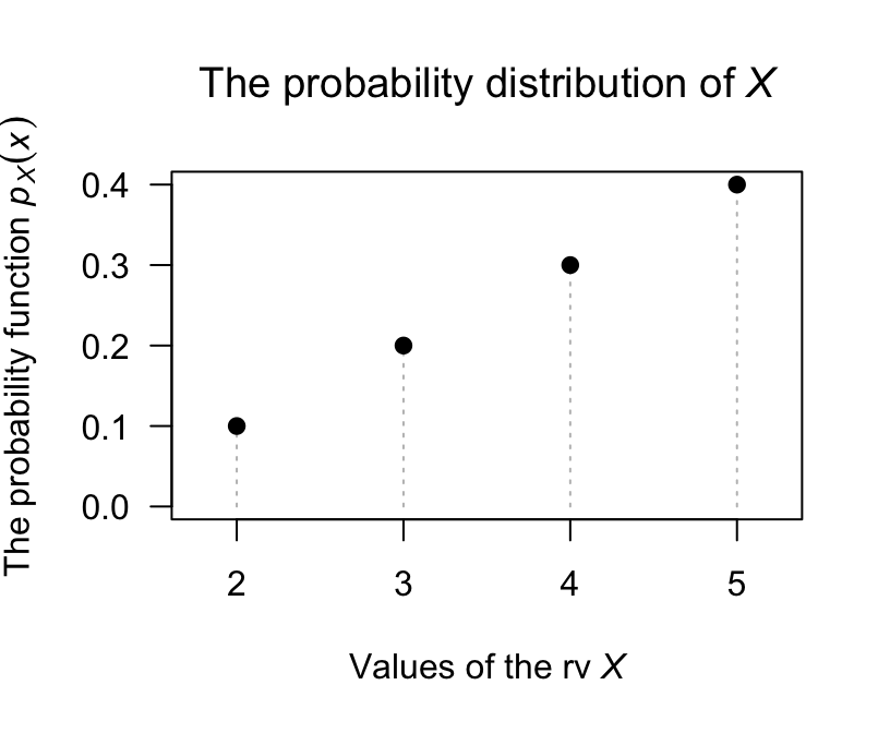
Figure 2.1: The probability function for the larger of two numbers drawn

Example 2.9 (Tossing heads) Suppose a fair coin is tossed twice, and the uppermost face is noted. Then the sample space is
\[ S = \{ (HH), (HT), (TH), (TT) \}. \] Let \(H\) be the number of heads observed. \(H\) is a (discrete) random variable, and the range of \(H\) is \(R_H = \{0, 1, 2\}\), representing the values that \(H\) can take.

The probability function maps each of these values to the associated probability. Using techniques from Chap. 1, the probabilities are:
\[\begin{align*} \Pr(H = 0) &= \Pr(\text{no heads}) = 0.25;\\ \Pr(H = 1) &= \Pr(\text{one head}) = 0.5;\\ \Pr(H = 2) &= \Pr(\text{two heads}) = 0.25. \end{align*}\] As a function, the probability function is
\[ p_H(h) = \Pr(H = h) = \begin{cases} 0.25 & \text{if $h = 0$};\\ 0.5 & \text{if $h = 1$};\\ 0.25 & \text{if $h = 2$};\\ 0 & \text{otherwise}. \end{cases} \] More succinctly,
\[ p_H(h) = \Pr(H = h) = \begin{cases} (0.5)0.5^{|h - 1|} & \text{for $h = 0$, $1$ or $2$};\\ 0 & \text{otherwise}. \end{cases} \] This information can also be presented as a table (Table 2.2) or graph (Fig. 2.2). Note that \(\sum_{t \in \{0, 1, 2\}} p_H(t) = 1\) and \(p_H(h)\ge0\) for all \(h\), as required of a pf.

Table 2.2: A table showing the distribution of \(H\), the number of heads in two tosses of a coin

\(h\)	0	1	2
\(\Pr(H = h)\)	0.25	0.5	0.25

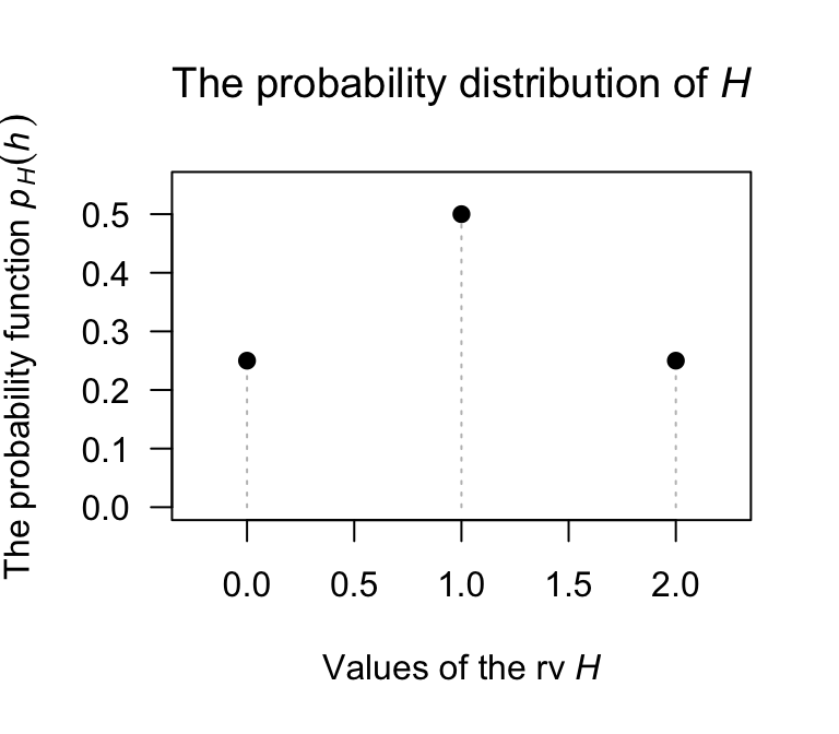
Figure 2.2: The probability function for \(H\), the number of heads on two tosses of a coin

2.3.2 Continuous random variables: Probability density functions

Using probability functions to describe the distribution of a continuous random variable is tricky, because probability behaves like mass at points. In the discrete case, mass can be distributed over a number (possibly countably infinite) of distinct points where each point has non-zero mass. However, in the continuous case, mass cannot be thought of as an attribute of a point but rather of a region surrounding a point.

The ideas from Example 1.20 are relevant here: The probability of throwing a cricket ball within two distances.

Definition 2.8 (Probability density function) The probability density function (pdf) of the continuous random variable \(X\) is a function \(f_X(\cdot)\) such that
\[ \Pr(a < X \le b) = \int_a^b f_X(x)\,dx \] for any interval \((a, b]\) (where \(a < b\)) on the real line.

We are usually only concerned with \(a, b\in R_X\), but it makes sense to think of the pdf as defined for all \(x\), insisting that \(f_X(x) = 0\) for \(x\notin R_X\). This definition states that areas under the graph of the pdf represent probabilities and leads to the following properties of the probability density function.

1. \(f_X(x) \ge 0\) for all \(-\infty < x < \infty\): The density function is never negative.
2. \(\displaystyle \int_{-\infty}^\infty f_X(x)\,dx = 1\): The total probability is one.
3. For an event \(E\) defined on a sample space \(S\), the probability of event \(E\) is computed using
   \[ \Pr(E) = \int_{E} f_X(x)\, dx. \]
4. Since exact values are not possible:
   \[\begin{align*} & \Pr(a < X \le b) = \Pr(a < X < b)\\ {} =& \Pr(a \le X < b) = \Pr(a \le X \le b) = \int_a^b f_X(x)\,dx \end{align*}\]

Properties 1 and 2 are sufficient to prove that a function is a pdf. That is, to show that some function \(g(x)\) is a pdf, showing that \(g(x) \ge 0\) for all \(-\infty < x < \infty\) and that \(\int_{-\infty}^\infty g(x)\,dx = 1\) is sufficient.

Property 4 results from noting that if \(X\) is a continuous random variable, \(\Pr(X = a) = 0\) for any and every value \(a\) for the same reason that a point has mass zero.

The value of a pdf at some point \(x\) does not represent a probability, but rather a probability density. Hence, the pdf can have any non-negative value of arbitrary size at a specific value of \(X\).

This last statement is easy to show. See Fig. 2.3, which shows some probability density function \(f(x)\). The probability of \(X\) occurring can be expressed as
\[ \Pr(X = x^*) \approx \Pr\left(x^* - \frac{\Delta x}{2} < X < x^* + \frac{\Delta x}{2} \right) \] as \(\Delta x \to 0\). This is shown by the shaded area, which can be approximated by the rectangle shown. That is,
\[\begin{align*} \Pr(X = x^*) &\approx \Pr\left(x^* - \frac{\Delta x}{2} < X < x^* + \frac{\Delta x}{2} \right) \\ &= \Delta x \times f(x). \end{align*}\] Rearranging,
\[ f(x) = \lim_{\Delta x \to 0} \frac{\Pr(X = x^*)}{\Delta x}. \] That is, the density function \(f(x)\) is not a probability.

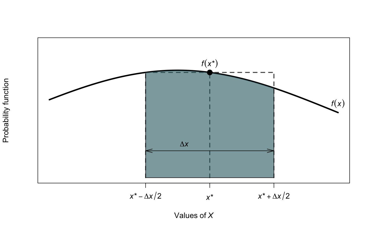
Figure 2.3: Finding probabilities for a continuous random variable \(X\)

Example 2.10 (Probability density function) Consider the continuous random variable \(W\) with the pdf
\[ f_W(w) = \begin{cases} 2w & \text{for $0 < w < 1$};\\ 0 & \text{elsewhere}. \end{cases} \] The probability \(\Pr(0 < W < 0.5)\) can be computed in two ways. One is to use calculus:
\[ \Pr(0 < W < 0.5) = w^2\Big|_0^{0.5} = 0.25. \] Alternately, the probability can be computed geometrically from the graph of the pdf (Fig. 2.4). The region corresponding to \(\Pr(0 < W < 0.5)\) is triangular; integration simply finds the area of this triangle. The area can also be found using the area of a triangle directly: the length of the base of the triangle, times the height of the rectangle, divided by two:
\[ 0.5 \times 1 /2 = 0.25, \] and the answer is the same as before.

Note that \(f_W(w)\) is greater than one for some values of \(w\). Since \(f_W(w)\) does not represent probabilities at each point (as \(W\) is continuous), this is not a problem. However, \(\int_{\mathbb{R}} f_W(w) \, dw = 1\) as required of a probability density.

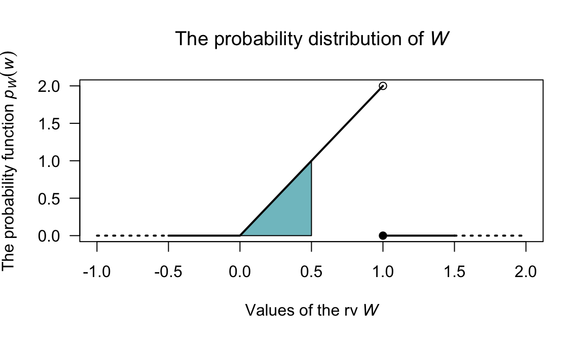
Figure 2.4: The probability function for \(W\)

2.3.3 Mixed random variables

Some random variables are neither continuous nor discrete, but have components of both. These random variables are called mixed random variables.

Example 2.11 (Mixed random variable) In a factory producing diodes, a proportion of the diodes \(p\) fail immediately. The distribution of the lifetime (in hundred of days), say \(Y\), of the diodes is given by a discrete component at \(y = 0\) for which \(\Pr(Y = 0) = p\), and a continuous part for \(y > 0\) described by
\[ f_Y(y) = (1 - p) \exp(-y) \quad \text{if $y > 0$.} \] Here, \(f_Y(y)\) is not itself a pdf as it doesn’t integrate to one; however the total probability is
\[ p + \int_0^\infty (1 - p)\exp(-y) \, dy = p + (1 - p) = 1 \] as required.

Consider a diode for which \(p = 0.4\). The probability distribution is displayed in Fig. 2.5 where a solid dot is included to show the discrete part. Representing the probability distribution in this mixed case is difficult, because of the need to combine a probability distribution and a pdf. These difficulties are overcome by using the distribution function (Sect. 2.4).

p <- 0.4
x <- seq(0, 4, 
         length = 100)
fy <- (1 - p) * exp( - x)
fy[1] <- 1 - p

Fy <- 0.4 + 0.6 * (1 - exp(-x ) )
F[1] <- p

plot(fy ~ x,
     lwd = 2,
     type = "l",
     xlim = c(-1, 4),
     xlab = expression(italic(Y)),
     ylab = expression(italic(f)[italic(y)](italic(y))),
     main = "Probability function",
     las = 1)
points( x = 0,
        y = 0.4,
        pch = 19)
points( x = 0,
        y = 0.6,
        pch = 1)

lines( x = c(-1, -0.5),
       y = c(0, 0),
       lwd = 2,
       lty = 2)
lines( x = c(-0.5, 0),
       y = c(0, 0),
       lwd = 2)
points( x = 0,
        y = 0,
        pch = 1)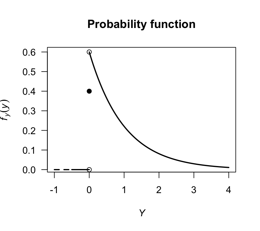

Figure 2.5: The probability function for the diodes example

2.4 The distribution function

Another way of describing random variables is using a distribution function (df), also called a cumulative distribution function (cdf). The df gives the probability that a random variable \(X\) is less than or equal to a given value of \(x\).

Definition 2.9 (Distribution function) For any random variable \(X\) the distribution function, \(F_X(x)\), is given by
\[ F_X(x) = \Pr(X \leq x) \quad \text{for $x\in\mathbb{R}$}. \]

The distribution function applies to discrete, continuous or mixed random variables. Importantly:

1. The definition includes a less than or equal to sign.
2. The distribution function is defined for all real numbers.

If \(X\) is a discrete random variable with range space \(R_X\), then the df is
\[\begin{align*} F_X(x) &= \Pr(X \leq x)\\ &= \sum_{x_i \leq x} \Pr(X = x_i)\text{ for }x_i\in R_X,\text{ and }-\infty < x < \infty. \end{align*}\] If \(X\) is a continuous random variable, the df is
\[\begin{align*} F_(x) &= \Pr(X \leq x)\\ &= \int^x_{-\infty} f(t)\,dt \text{ for } -\infty < x < \infty. \end{align*}\]

Example 2.12 (Tossing heads) Consider the simple example in Example 2.9 where a coin is tossed once. The probability function for \(H\) is given in that example in numerous forms. To determine the df, first note that when \(h < 0\), the accumulated probability is zero; hence, \(F_H(h) = 0\) when \(h < 0\). At \(h = 0\), the probability of \(0.25\) is accumulated all at once, and no more probability is accumulated until \(h = 1\). Thus, \(F_H(h) = 0.25\) for \(0 \le h < 1\). Continuing, the df is
\[ F_H(h) = \begin{cases} 0 & \text{for $h < 0$};\\ 0.25 & \text{for $0\le h < 1$};\\ 0.75 & \text{for $1\le h < 2$};\\ 1 & \text{for $h\ge 2$}. \end{cases} \] The df can be displayed graphically, being careful to clarify what happens at \(H = 1\), \(H = 2\) and \(H = 3\) using open or filled circles (Fig. 2.6).

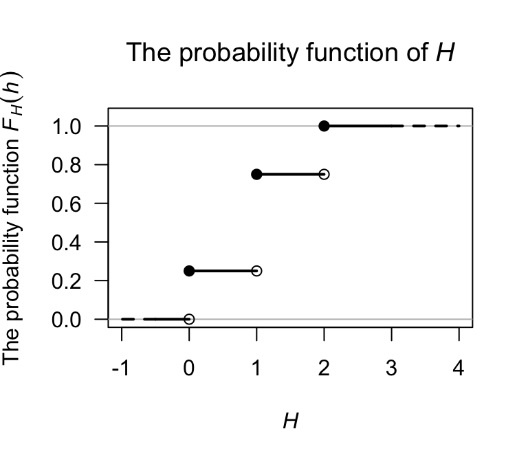
Figure 2.6: A graphical representation of the distribution function for the tossing-heads example. The filled circles contain the given point, while the empty circles omit the given point.

Example 2.13 (Probability function) Consider a continuous random variable \(V\) with pdf
\[ f_V(v) = \begin{cases} v/2 & \text{for $0 < v < 2$};\\ 0 & \text{otherwise.} \end{cases} \] The df is zero whenever \(v\le 0\). For \(0 < v < 2\),
\[ F_V(v) = \int_0^v t/2\,dt = v^2/4. \] Whenever \(v\ge 2\), the df is one. So the df is
\[ F_V(v) = \begin{cases} 0 & \text{if $v\le 0$};\\ v^2/4 & \text{if $0 < v < 2$};\\ 1 & \text{if $v\ge 2$.} \end{cases} \] A picture of the df is shown in Fig. 2.7.

par(mfrow = c(1, 2))

fv <- function(v){
  y <- array( 0, dim = length(v))
  fy <- ifelse( (v > 0) & ( v < 2 ),
                v/2,
                0)
  fy
}

v <- seq(-2, 4, 
         length = 100)
plot(fv(v) ~ v,
     type = "l",
     lwd = 2,
     las = 1,
     xlab = expression(italic(v)),
     ylab = "Probability function",
      main = expression(paste("The probability function for"~italic(V))),
)


vb <- seq(0, 2,
         length = 100)
vbDF <- ( vb ^ 2 ) / 4

plot( x = c(-2, 4),
      y = c(0, 1),
      type = "n",
      main = expression(paste("The distribution function for"~italic(V))),
      xlab = expression(italic(v)),
      ylab = "Distribution function",
      las = 1)
lines( x = c(-2, -1),
       y = c(0, 0),
       lwd = 3,
       lty = 2)
lines( x = c(-1, 0),
       y = c(0, 0),
       lwd = 3,
       lty = 1)
lines( vbDF ~ vb,
       lwd = 3)
lines( x = c(2, 3),
       y = c(1, 1),
       lwd = 3)
lines( x = c(3, 4),
       y = c(1, 1),
       lwd = 3,
       lty = 2)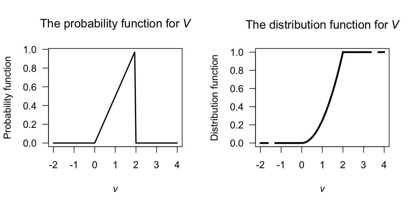

Figure 2.7: The probability function (left) and the distribution function (right) for \(V\)

For the integral, do not write
\[ \int_0^v v/2\,dv. \] It makes no sense to have the variable of integration as a limit on the integral and also in the function to be integrated. Either write the integral as given in the example, or write \(\int_0^t v/2\,dv = t^2/4\) and then change the variable from \(t\) to \(v\).

Properties of the df are stated below.

1. \(0\leq F_X(x)\leq 1\) because \(F_X(x)\) is a probability.
2. \(F_X(x)\) is a non-decreasing function of \(x\). That is, if \(x_1 < x_2\) then \(F_X(x_1) \leq F_X(x_2)\).
3. \(\displaystyle{\lim_{x\to \infty} F_X(x)} = 1\) and \(\displaystyle{\lim_{x\to -\infty} F_X(x)} = 0\).
4. \(\Pr(a < X \leq b) = F_X(b) - F_X(a)\).
5. If \(X\) is discrete, then \(F_X(x)\) is a step-function. If \(X\) is continuous, then \(F_X\) will be a continuous function for all \(x\).

We have seen how to find \(F_X(x)\) given \(\Pr(X = x)\), or to find \(F_X(x)\) given \(f_X(x)\). But can we proceed in the other direction too? That is, given \(F_X(x)\), how do we find \(\Pr(X = x)\) for \(X\) discrete, or \(f_X(x)\) for \(X\) continuous?

As seen from the graph of the df in Example 2.12, the values of \(x\) where a ‘jump’ in \(F_X(x)\) occurs are the points in the range space, and the probability associated with a particular point in \(R_X\) is the ‘height’ of the jump there. That is,
\[\begin{equation} p_X(x_j) = \Pr(X = x_j) = F_X(x_j) - F_X(x_{j - 1}). \end{equation}\]

For \(X\) continuous, from the Fundamental Theorem of Calculus,
\[\begin{equation} f_X(x) = \frac{dF_X(x)}{dx} \quad \text{where the derivative exists.} \tag{2.1} \end{equation}\]

Example 2.14 (Distribution function) Consider the df
\[ F_X(x) = \begin{cases} 0 & \text{for $x < 0 $};\\ x(2 - x) & \text{for $0 \le x \le 1$};\\ 1 & \text{for $x > 1$.} \end{cases} \] To find the pdf, use Eq. (2.1):
\[ f_X(x) = \begin{cases} \frac{d}{dx} 0 & \text{for $x < 0 $};\\ \frac{d}{dx} x(2 - x) & \text{for $0 \le x \le 1$};\\ \frac{d}{dx} 1 & \text{for $x > 1$} \end{cases} = \begin{cases} 0 & \text{for $x < 0 $};\\ 2(1 - x) & \text{for $0 \le x \le 1$};\\ 0 & \text{for $x > 1$} \end{cases} \] which is usually written as \(f_X(x) = 2(1 - x)\) for \(0 < x < 1\), and \(0\) elsewhere.

For mixed random variables, representing the probability distribution can be tricky because we need to combine a probability distribution and a pdf. These difficulties are overcome by using the distribution function.

Example 2.15 (Mixed random variable) For the diode example (Example 2.11), the df of \(Y\) is (Fig. 2.8):
\[ F_Y(y) = \begin{cases} 0 & \text{if $y < 0$}\\ 0.4 & \text{if $y = 0$}\\ 0.4 + 0.6(1 - \exp(-y)) & \text{if $y > 0$}. \end{cases} \]

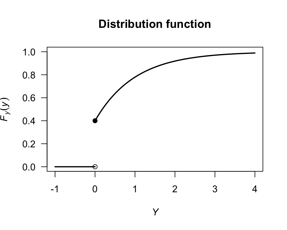
Figure 2.8: The distribution function for the diodes example

2.5 Exercises

Exercise 2.1 For the following random processes, determine the range space \(R_X\) and define the random variable of interest. Determine whether the random variable is discrete, continuous or mixed. Justify your answer.

1. The number of heads in two throws of a fair coin.
2. The number of throws of a fair coin until a head is observed.
3. The time taken to download a webpage.
4. The time it takes to walk to work.
5. The number of cars that pass through an intersection during a day.
6. The number of X-rays taken at a hospital per day.
7. The barometric pressure in a given city at \(5\)pm each afternoon.

Exercise 2.2 The random variable \(X\) has the pf
\[ p_X(x) = \begin{cases} 0.3 & \text{for $x = 10$};\\ 0.2 & \text{for $x = 15$};\\ 0.5 & \text{for $x = 20$};\\ 0 & \text{elsewhere}. \end{cases} \]

1. Find and plot the distribution function for \(X\).
2. Compute \(\Pr(X > 13)\).
3. Compute \(\Pr(X \le 10 \mid X\le 15)\).

Exercise 2.3 Consider the continuous random variable \(Z\) with pdf
\[ f_Z(z) = \begin{cases} 2(3 - z)/15 & \text{for $-1 < z < 2$};\\ 0 & \text{elsewhere}. \end{cases} \]

1. Find and plot the df of \(Z\).
2. Find \(\Pr(Z < 0)\).

Exercise 2.4 Consider the discrete random variable \(W\) with df
\[ F_W(w) = \begin{cases} 0 & \text{for $w < 10$};\\ 0.3 & \text{for $10 \le w < 20$};\\ 0.7 & \text{for $20 \le w < 30$};\\ 0.9 & \text{for $30 \le w < 40$};\\ 1 & \text{for $w \ge 40$}. \end{cases} \]

1. Find and plot the pmf of \(W\).
2. Compute \(\Pr(W < 25)\) using the pmf, and using the df.

Exercise 2.5 Consider the continuous random variable \(Y\) with df
\[ F_Y(y) = \begin{cases} 0 & \text{for $y \le 0$};\\ y(4 - y^2)/3 & \text{for $0 < y < 1$};\\ 1 & \text{for $y \ge 1$}. \end{cases} \]

1. Find and plot the pdf of \(Y\).
2. Compute \(\Pr(Y < 0.5)\) using the pdf and using the df.

Exercise 2.6 A study of the service life of concrete in various conditions (Liu and Shi 2012) used the following distribution for the chlorine threshold of concrete¹:
\[ f(x; a, b, c) = \begin{cases} \frac{2(x - a)}{(b - a)(c - a)} & \text{for $a\le x\le c$};\\[6pt] \frac{2(b - x)}{(b - a)(b - c)} & \text{for $c\le x\le b$};\\ 0 & \text{otherwise}, \end{cases} \] where \(c\) is the mode, and \(a\) and \(b\) are the lower and upper limits.

1. Show that the distribution is a valid pdf.
2. Previous studies, cited in the article, suggest the values \(a = 0.6\) and \(c = 5\), and that the distribution is symmetric. Write down the pdf for this case.
3. Determine the df using the values above.
4. Plot the pdf and df.
5. Determine \(\Pr(X > 3)\).
6. Determine \(\Pr(X > 3 \mid X > 1)\).
7. Explain the difference in meaning for the last two answers.

Exercise 2.7 In a study modelling waiting times at a hospital (Khadem et al. 2008), patients are classified into one of three categories:

• Red: Critically ill or injured patients.
• Yellow: Moderately ill or injured patients.
• Green: Minimally injured or uninjured patients.

For ‘Yellow’ patients, the service time of doctors are modelled using a triangular distribution, with a minimum at \(3.5\) mins, a maximum at \(30.5\) mins and a mode at \(5\) mins.

1. Plot the pdf and df.
2. If \(S\) is the service time, compute \(\Pr(S > 20 \mid S > 10)\).

Exercise 2.8 In meteorological studies, rainfall is often graphed using rainfall exceedance charts (Dunn 2001): the plotted function is \(1 - F_X(x)\) (also called the survivor function in other contexts), where \(X\) represents the rainfall.

1. Explain what is measured by \(1 - F_X(x)\) in this context, and explain why it may be more useful than just \(F_X(x)\) when studying rainfall.
2. The data in Table 2.3 shows the total monthly rainfall at Charleville, Queensland, from 1942 until 2022 for the months of June and December. (Data supplied by the Bureau of Meteorology.) Plot \(1 - F_X(x)\) for this rainfall data for each month on the same graph.
3. Suppose a producer requires at least \(50\) mm of rain in June to plant a crop. Find the probability of this occurring from the plot above.
4. Determine the median monthly rainfall in Charleville in June and December.
5. Decide if the mean or the median is an appropriate measure of central tendency, giving reasons for your answer.
6. Compare the probabilities of obtaining \(30\) mm, \(50\) mm, \(100\) mm and \(150\) mm of rain in the months of June and December.
7. Write a one-or two-paragraph explanation of how to use diagrams like that presented here. The explanation should be aimed at producers (that is, experts in farming, but not in statistics) and should be able to demonstrate the usefulness of such graphs in decision making. Your explanation should be clear and without jargon. Use diagrams if necessary.

Table 2.3: The monthly rainfall in Charleville, in mm, from 1942 to 2022: The number of months with the indicated rainfall

	June	December
Zero rainfall	3	0
Over 0 to under 20	41	17
20 to under 40	19	17
40 to under 60	12	21
60 to under 80	2	9
80 to under 100	2	6
100 to under 120	0	3
120 to under 140	2	1
140 to under 160	0	4
160 to under 180	0	0
180 to under 200	0	1
200 to under 220	0	1

Exercise 2.9 Five people, including you and a friend, line up at random. The random variable \(X\) denotes the number of people between yourself and your friend. Determine the probability function of \(X\).

Exercise 2.10 Let \(Y\) be a continuous random variable with pdf
\[ f_Y(y) = a(1 - y)^2,\quad \text{for $0\le y\le 1$}. \]

1. Show that \(a = 3\).
2. Find \(\Pr\left(| Y - \frac{1}{2}| > \frac{1}{4} \right)\).
3. Use R to draw a graph of \(f_Y(y)\) and show the area described above.

Exercise 2.11 Consider the function
\[ p(x) = \begin{cases} \log_{10}\left(1 + \frac{1}{x} \right),& \text{for $x = 1, 2, 3, \dots, 9$}\\ 0 & \text{otherwise}. \end{cases} \]

1. Show that \(p(x)\) is a probability function.
2. Determine an expression for the corresponding distribution function.

Exercise 2.12 Quartic polynomials are sometimes used to model mortality (e.g., Fitzpatrick and Moore (2018)). Suppose the model
\[ f_Y(y) = k y^2 (100 - y)^2\quad \text{for $0 \le y \le 100$} \] (for some value of \(k\)) is used for describing mortality where \(Y\) denotes age at death in years. Using this model, is a person more likely to die at age between \(60\) and \(70\) or live past \(70\)?

Exercise 2.13 To detect disease in a population through a blood test, usually every individual is tested. If the disease is uncommon, however, an alternative method is often more efficient.

In the alternative method (called a pooled test), blood from \(n\) individuals is combined, and one test is conducted. If the test returns a negative result, then none of the \(n\) people have the disease; if the test returns a positive result, all \(n\) individuals are then tested individually to identify which individual(s) have the disease.

Suppose a disease occurs in an unknown proportion of people \(p\) of people. Let \(X\) be the number of tests to be performed for a group of \(n\) individuals using the pooled test approach.

1. Determine the sample space for \(X\).
2. Deduce the probability distribution of the random variable \(X\).

Exercise 2.14 In a deck of cards, consider an Ace as high, and all picture cards (i.e., Jacks, Queens, Kings, Aces) as worth ten points. All other cards are worth their face value (i.e., a 8 is worth eight points.)

Deduce the probability distribution of the absolute difference between the value of two cards drawn at random from a well-shuffled deck of \(52\) cards.

Exercise 2.15 The leading digits of natural data that span many orders of magnitude (e.g., lengths of rivers; populations of countries) often follow Benford’s law. Numbers are said to satisfy Benford’s law if the leading digit, say \(d\) (for \(d\in \{1, \dots, 9\}\)) has the probability mass function
\[ p_D(d) = \log_{10}\left( \frac{d + 1}{d} \right). \]

1. Plot the probability mass function of \(D\).
2. Compute and plot the distribution function of \(D\).

Exercise 2.16 Consider the random variable \(X\) with pdf
\[ f(x) = \begin{cases} \frac{k}{\sqrt{x(1 - x)}} & \text{for $0 < x < 1$};\\ 0 & \text{elsewhere}. \end{cases} \]

1. Plot the density function.
2. Determine, and then plot, the distribution function.

Exercise 2.17 Consider the distribution function
\[ F_X(x) = \begin{cases} 0 & \text{for $x < 0$};\\ \exp(-1/x) & \text{$x \ge 0$}. \end{cases} \]

1. Show that this is a valid df.
2. Compute the pdf.
3. Plot the df and pdf.

Exercise 2.18 Suppose a dealer deals four cards from a standard \(52\)-card pack. Define \(Y\) as the number of suits in the four cards. Deduce the distribution of \(Y\).

---

Peter K. Dunn, 2024: CC BY-NC-SA 4.0