1 Probability essentials

Upon completion of this module you should be able to:

• understand the concepts of probability, and apply rules of probability.
• define probability from using different methods and apply them to compute probabilities in various situations.
• apply the concepts of conditional probability and independence.
• differentiate between mutually exclusive events and independent events.
• apply Bayes’ Theorem.
• use combinations and permutations to compute the probabilities of various events involving counting problems.

1.1 Introduction

Imagine if life was deterministic! The commute to the gym, university or work would always take exactly the same length of time; weather predictions would always be accurate; you would know exactly what lotto numbers would be drawn on the weekend…

However, life is full of unpredictable variation.

Variation may be unpredictable, but patterns still emerge. We may not know what the next toss of a coin will produce… but we see a pattern in the long run: a Head appears about half the time.

Probability is one of the tools used to describe and understand this unpredictability. Distribution theory is about describing the patterns in this unpredictability using probability. Statistics is about data collection and extracting information from data, using probability and distribution theory.

In most fields of study, situations exist where being certain is almost impossible, and so probability is necessary:

• What is the chance that a particular share price will crash next month?
• What are the odds that a medical patient will suffer from a dangerous side-effect?
• How likely is it that a dam will overflow next year?
• What is the chance of finding a rare bird species in a given forest?

To answer these questions, a framework is needed: concepts like probability need defining, and notation and theory are required. These tools are important for modelling real-world phenomena, but also for providing a firm mathematical foundation for the theory of statistics.

This chapter covers the concept of probability, introduces notation and definitions, and develops some theory useful in working with probabilities.

1.2 Sets and sample spaces

The basis of probability is working with sets, which we first define.

Definition 1.1 (Sets) A set is an unordered collection of distinct elements, usually denoted using a capital letter: \(A\).

The order of the elements in the set is not relevant (‘unordered’). Any elements that are repeated are irrelevant.

Sets may comprise:

• Elements that are distinct, such as the set comprising the six states of Australia.
• Elements that represent regions, such as the heights of people.

Definition 1.2 (Elements) Distinct elements of a set \(A\) are usually denoted by lower-case letters, and are shown to belong to a set by enclosing them in braces: \[ A = \{ a_1, a_2, a_3, a_4\}. \] If the element \(a_j\) is in the set \(A\), we write \(a_j \in A\) (where \(\in\) can be read as ‘is an element of’).

Example 1.1 (Sets) Define the set \(S\) as the ‘set of suits in a standard pack of cards’. Then, \(S = \{\clubsuit, \spadesuit, \heartsuit, \diamondsuit\}\). We can write that \(\spadesuit \in S\).

Example 1.2 (Sets) These three sets are all equivalent: \[\begin{align*} A &= \{\text{Brisbane}, \text{Sydney}, \text{Hobart}\};\\ B &= \{\text{Hobart}, \text{Brisbane}, \text{Sydney}\};\\ C &= \{\text{Brisbane}, \text{Sydney}, \text{Hobart}, \text{Sydney}, \text{Hobart} \};\\ \end{align*}\]

A set with no elements is given a special name: the empty set.

Definition 1.3 (Empty set) The null set, or the empty set, has zero elements, and is denoted by \(\emptyset\).

Sets are related to the outcomes of random processes (or random experiments).

Definition 1.4 (Random process) A random process is a procedure that:

• can be repeated, in theory, indefinitely under essentially identical conditions; and
• has well-defined outcomes; and
• the outcome of any individual repetition is unpredictable.

Examples of simple random processes include tossing a coin, or rolling a die. While the outcome of any instance of a random process produces is unknown, usually the possible outcomes are known. The possible outcomes of the random process constitute a special set, called the sample space.

Definition 1.5 (Sample space) A sample space (or event space, or outcome space) for a random process is a set of all possible outcomes from a random process, usually denoted by \(S\), \(\Omega\) or \(U\) (for the ‘universal set’).

Example 1.3 (Sample Space) Consider rolling a die. The sample space is the set of all possible outcomes: \[ S = \{ 1, 2, 3, 4, 5, 6\}. \]

1.3 Describing sets and elements

Sets can be described in various ways:

• by enumerating the individual elements, either directly, using a description, or by stating a pattern.
• by describing what is common to all elements of the set.
• by using a rule.

The number of elements in a set (the cardinality) can be:

• finite (informally, the elements can be counted);
• countable infinite (informally, the elements could be counted in principle… but there are an infinite number of them); or
• infinite (informally, there are too many elements to count).

In sets with a finite or countably infinite number of elements, a single element of \(S\) is called an element or sample point. To denote that a certain element, say \(a_1\), belongs to a set, say \(A\), write \(a_1\in A\).

Example 1.4 (Sets) Define set \(B\) as ‘the even numbers after rolling a single die’. The sample space is (Example 1.3) \(S = \{ 1, 2, 3, 4, 5, 6\}\). \(B\) can also be described by listing the elements: \(B = \big\{\) ⚁, ⚃, ⚅\(\big\}\). \(B\) contains a finite number of elements.

The set \(N\) of odd numbers could be defined by enumeration, by giving a pattern: \(N = \{1, 3, 5, 7, 9, \dots\}\). \(N\) contains a countably infinite number of elements.

Set \(A\) can be defined by describing the elements: \(A = \left\{\right.\)Countries whose names begin and end with the letter ‘A’\(\left.\right\}\). The elements of \(A\) include, for example, ‘Austria’, ‘Antigua and Barbuda’ and ‘Albania’. \(A\) contains a finite number of elements.

The set \(R\) refers to the positive real numbers, and can be defined by a rule: \(R = \{ x \mid x > 0\}\), where the notations means ‘the set \(R\) consists of elements \(x\) such that all values of \(x\) are greater than zero’. (The symbol \(\mid\) is read as ‘such that’.) \(R\) contains an infinite number of elements.

Example 1.5 (Throwing a cricket ball) Consider throwing a cricket ball, where the distance of the throw is of interest. The set \(D\) of possible distances is \(D = \{ d \mid d > 0 \}\). \(D\) has an infinite number of elements.

Sets do not have to be one-dimensional. We could define the set \(P\) as \(P = \{(x, y) \mid \text{$0 < x < 1$ and $0 < y < 1$} \}\), which defines a unit square on the Cartesian axes.

1.4 Operations on sets

Various operations are defined for sets.

Definition 1.6 (Intersection, union, subset, complement) Consider two sets \(A\) and \(B\) defined on the same sample space \(S\).

• The intersection of sets \(A\) and \(B\), written as \(A\cap B\), is the set of points in both \(A\) and \(B\). We say \(A\) and \(B\).
• The union of sets \(A\) and \(B\), written as \(A\cup B\), is the combined set of all the points in either \(A\) or \(B\), or both. (Usually we just say that \(A\cup B\) comprises the points in ‘\(A\) or \(B\)’.) We say \(A\) or \(B\).
• \(A\) is a subset of \(B\), written as \(A\subset B\), if all the elements of \(A\) are in \(B\). (Set \(B\) may have other elements that are not in \(A\).) This definition requires that \(A\) has fewer elements than \(B\). We write \(A\subseteq B\) if \(A\) is a subset of \(B\) or is equivalent to \(B\) (and so \(A\) and \(B\) may have the same number of elements).
• The complement of \(A\), written \(\overline{A}\), is the set of points in \(S\) but not in \(A\).

The visual representation in Fig. 1.1 may help clarify.

Be aware of variations in notation! Other notation for the complement of an event \(A\) (everything not in event \(A\)) is \(\overline{A}\), or \(A^c\), or \(A'\).

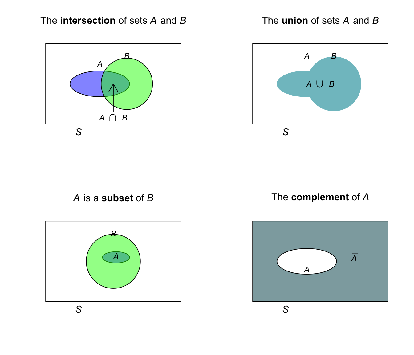
FIGURE 1.1: Intersection, union, subsets, and complement of sets. The rectangle represents the universal set, \(S\).

Example 1.6 (Relationships between sets) Suppose we define these sets: \[\begin{align*} C &= \{ 0, 1, 2, 3, 4, 5\};\\ D &= \{ 4, 5, 6, 7\};\\ E &= \{ 6 \}. \end{align*}\] Then: \[\begin{align*} C \cap D &= \{ 4, 5\}; & C \cup D &= \{ 0, 1, 2, 3, 4, 5, 6, 7\};\\ E &\in D; & E &\notin C;\\ C \cap E &= \emptyset; & D \cap E &= D. \end{align*}\]

1.5 Special sets of numbers

Some special sets of numbers are useful to define:

• Natural (or counting) numbers are denoted \(\mathbb{N}\): \(\{1, 2, 3, \dots\}\).
• Integers are denoted \(\mathbb{Z}\): \(\{\ldots, -2, 1, 0, 1, 2, 3, \dots\}\).
• Rational numbers are denoted \(\mathbb{Q}\).
• Real numbers are denoted \(\mathbb{R}\).
• Positive real numbers are denoted \(\mathbb{R}_{+}\).
• Negative real numbers are denoted \(\mathbb{R}_{-}\).
• Complex numbers are denoted \(\mathbb{C}\).

Example 1.7 (Sets) We could write \(\mathbb{Q} = \{m/n \mid m, n \in \text{$\mathbb{Z}$ and $n\ne 0$}\}\).

We can also write \(\mathbb{Z} \in \mathbb{R}\), but \(\mathbb{R} \notin \mathbb{Z}\).

We can define \(\mathbb{N}_0 = \{ 0 \cup \mathbb{N}\}\).

1.6 Events

While the sample space defines the set of all possible outcomes, usually we are interested in just some of those elements of the sample space.

Definition 1.7 (Event) An event \(E\) is a subset of \(S\), and we write \(E \subseteq S\).

By this definition, \(S\) itself is an event. If the sample space has a finite or countable infinite number of elements, then an event is a collection of sample points.

Example 1.8 (Events) Consider the simple random process of tossing a coin twice. The sample space is: \[ S = \{(HH), (HT), (TH), (TT) \}, \] where \(H\) represents tossing a head and \(T\) represents tossing a tail, and the pair lists the result of the two toss in order.

We can define the event \(A\) as ‘tossing a head on the second toss’, and list the elements: \[ A = \{ (HH), (TH)\}. \] The event ‘the set of outcomes corresponding to tossing three heads’ is the null or empty set; no sample points have three heads.

Definition 1.8 (Elementary event) In a sample space with a finite or countable infinite number of elements, an elementary event (or a simple event) is an event with one sample point, that cannot be decomposed into smaller events.

A collection of elementary events is sometimes called a compound event.

Example 1.9 (Elementary and compound events) Consider observing the outcome on a single roll of a die (Example 1.11). The elementary events are:
\[\begin{align*} E_1:&\quad \text{Roll a 1}; & E_2:&\quad \text{Roll a 2};\\ E_3:&\quad \text{Roll a 3}; & E_4:&\quad \text{Roll a 4};\\ E_5:&\quad \text{Roll a 5}; & E_6:&\quad \text{Roll a 6}.\\ \end{align*}\]

Define the event \(T\) as ‘numbers divisible by \(3\)’ and event \(D\) as ‘numbers divisible by \(2\)’. \(T\) and \(D\) are compound events: \[ T = \{3, 6 \} \quad \text{and} \quad D = \{2, 4, 6 \}. \]

An important concept is that of an occurrence of an event.

Definition 1.9 (Occurrence) An event \(A\) occurs on a particular trial of a random process if the outcome of the trial is part of the sample space for the random process.

Example 1.10 Consider events \(T\) and \(D\) defined in Example 1.9. For these events: \[ T\cap D = \{ 6 \};\qquad\text{and}\qquad T\cup D = \{2, 3, 4, 6\}. \]

Definition 1.10 (Mutually exclusive) Events \(A\) and \(B\) are mutually exclusive if, and only if, \(A\cap B = \emptyset\); that is, they have no elements in common.

The term disjoint is used for sets, whereas mutually exclusive is used when referring to events.

Example 1.11 (Rolling a die) Suppose we roll a single, six-sided die. For rolling a die, the sample space is \(S = \{1, 2, 3, 4, 5, 6\}\).

We can define these two events:
\[\begin{align*} E &= \text{An even number is thrown} & &= \{2, 4, \phantom{5, }6\};\\ G &= \text{A number larger than 3 is thrown} & &= \{\phantom{2, }4, 5, 6\}. \end{align*}\] Then,
\[\begin{align*} E \cap G &= \{4, 6\} & E \cup G &= \{ 2, 4, 5, 6\}\\ \overline{E} &= \{ 1, 3, 5\} & \overline{G} &= \{ 1, 2, 3\}. \end{align*}\] We make other observations too:
\[\begin{align} E \cap \overline{G} &= \{2, 4, 6\} \cap \{ 1, 2, 3\} = \{ 2 \};\\ \overline{E} \cap \overline{G} &= \{1, 3, 5\} \cap \{ 1, 2, 3\} = \{ 1, 3 \}. \end{align}\] See Fig. 1.2

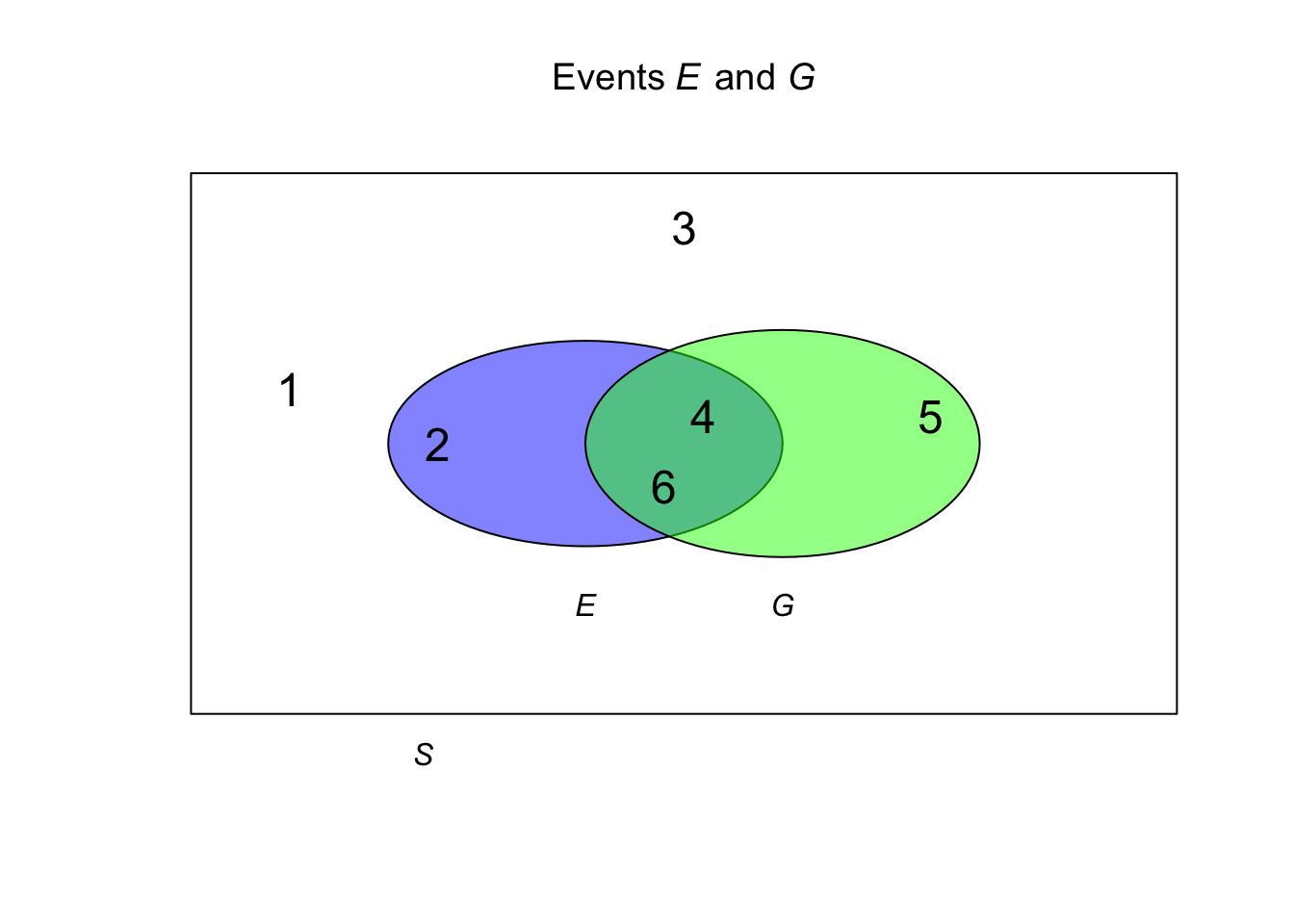
FIGURE 1.2: Events \(E\) and \(G\)

Example 1.12 (Tossing a coin twice) Consider the simple random process of tossing a coin twice (Example 1.8), and define events \(M\) and \(N\) as follows:

Event	Notation	Set
‘Obtain a Head on Toss 1’	\(M\)	\(\{(HT), (HH)\}\)
‘Obtain a Tail on Toss 1’	\(N\)	\(\{(TT), (TH)\}\)

The two sets are disjoint, as there are no sample points in common. The events are therefore mutually exclusive.

Set algebra has many rules; we only provide some. For sets \(A\), \(B\) and \(C\) defined on the same sample space, these rules are defined:

• Commutative: \(A\cup B = B \cup A\).
• Associative: \(A\cup(B\cup C) = (A\cup B)\cup C\).
• Distributive: \(A\cap (B\cup C) = (A\cap B)\cup (A \cap C)\).
• De Morgan’s law: \(\overline{A \cap B } = \overline{A} \cup \overline{B}\).
• De Morgan’s law: \(\overline{A \cup B } = \overline{A} \cap \overline{B}\).

Proof. These may be proved using the rules of probability (given later), or using Venn diagrams.

Example 1.13 (Throwing a cricket ball) Consider throwing a cricket ball, where the distance of the throw is of interest (Example 1.5), so that \(D\) is the set of possible distances: \(D = \{ d \mid d > 0 \}\).

We can define these two events:
\[\begin{align*} B_1:&\quad \text{Throw a cricket ball at least $40$m} &&= [40, \infty);\\ B_2:&\quad \text{Throw a cricket ball less than $50$m} &&= (0, 50). \end{align*}\] The notation for \(B_1\) means that a distance of \(40\) m is included in \(B_1\). The notation for \(B_2\) means that distances of \(0\) m and \(50\) m are not included in \(B_2\).

Then:
\[\begin{align*} B_1 \cap B_2 &= \text{Throw the ball at least $40$m but less than $50$m};\\ B_1 \cup B_2 &= \mathbb{R}_+;\\ \overline{B_1} &= \text{Throw the ball less than $40$m}. \end{align*}\]

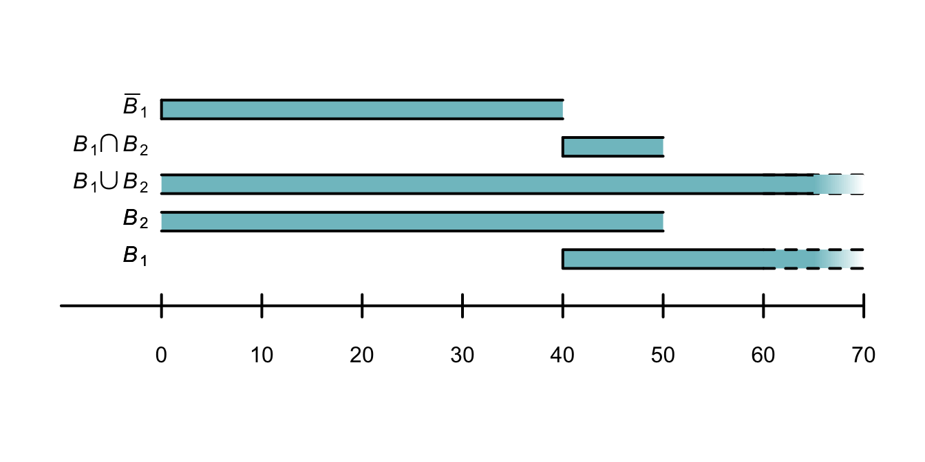
FIGURE 1.3: The two events \(B_1\) and \(B_2\) defined for throwing a cricket ball

1.7 Assigning probabilities: discrete events

The chance of an event occurring is formalised by assigning a number, called a probability, to an event. We denote the probability of an event \(E\) occurring as \(\text{Pr}(E)\).

Be aware of variations in notation! The probability of an event \(E\) occurring can be denoted as \(\text{P}(E)\), \(\text{Pr}(E)\), \(\text{Pr}\{E\}\), or using other similar notation.

A probability of \(0\) is assigned to an event that never occurs (i.e., corresponds to the empty set), and \(1\) to an event that is certain to occur (i.e., corresponds to the universal set). This method is appealing as it aligns with the idea of proportions as numbers between \(0\) and \(1\).

Developing a method of assigning sensible probabilities to events is difficult. Four methods are discussed here.

Sometimes, the chance of an event occurring is expressed as odds, which are not the same as probabilities. Odds are the ratio of how often an event is likely to occur, to how often the event is likely to not occur.

Using odds, an impossible event is assigned \(0\), a certain event is assigned \(\infty\), and an event that will happen just as often as not happen is assigned \(1\).

We will only use the system with probabilities between \(0\) and \(1\) in this book.

Importantly: ‘odds’ and ‘probability’ are not the same.

1.7.1 Empirical (relative frequency) approach

When a random process is repeated many times, counting the number of times the event of interest occurs means we can compute the proportion of times the event occurs. Mathematically, if the random process is repeated \(n\) times, and event \(E\) occurs in \(m\) of these (\(m < n\)), then the probability of the event occurring is \[ \Pr(E) = \lim_{n\to\infty} \frac{m}{n}. \] In practice, \(n\) needs to be very large—and the repetitions random—to compute probabilities accurately, and approximate probabilities can only ever be found (since \(n\) is finite in practice).

This is the empirical (or relative frequency) approach to probability.

This method cannot always be used in practice. Consider the probability that the air bag in a car will prevent a serious injury to the driver. It is not ethical or financially viable to crash thousands of vehicles with drivers in them to see how many break bones. Fortunately, car manufacturers use dummies to represent people, and crash small numbers of cars to get some indications of the probabilities. In these situations, sometimes computer simulations can be used to approximate the probabilities.

Example 1.14 (Salk vaccine) In 1954, Jonas Salk developed a vaccine against polio (Williams (1994), 1.1.3). To test the effectiveness of the vaccine, the data in Table 1.1 were collected.

The relative frequency approach can be used to estimate the probabilities of developing polio with the vaccine and without the vaccine (the control group):
\[\begin{align*} \Pr(\text{develop polio in control group}) &\approx \frac{115}{201\,229} = 0.000571;\\[3pt] \Pr(\text{develop polio in vaccinated group}) &\approx \frac{33}{200\,745} = 0.000164, \end{align*}\] where ‘\(\approx\)’ means ‘approximatey equal to’. The estimated probability of contracting polio in the control group is about 3.5 times greater than in the control group. The precision of these sample estimates could be quantified by producing a confidence interval for the proportions.

TABLE 1.1: The number of paralytic cases for two groups of children: one group of controls and another vaccinated with the Salk polio vaccine

	Number treated	Paralytic cases
Vaccinated	200 745	33
Control	201 229	115

Example 1.15 (Simulating a coin toss) Repeating random processes large numbers of times can be impractical and tedious. However, sometimes a computer can be used to simulate the random processes. Consider using a computer to simulate large numbers of coin tosses; here, R is used to simulate 500 tosses.

Use \(\Pr(\text{Toss head}) = 0.5\). Then, after each toss, the probability of obtaining a head using all the available information was computed after each toss. For one such simulation, these running probabilities are shown in Fig. 1.4. While the result of any single toss is unpredictable, we see the general pattern emerging: Heads occur about half the time.

NumTosses <- 500 # Simulated tossing a coin 500 times
Tosses <- sample(x = c("H", "T"),    # Choose "H"  or  "T"
                 size = NumTosses,   # Do this 500 times
                 replace = TRUE)     # H and T can be reselected 
Tosses[1 : 10]                       # Show the first 10 results
#>  [1] "T" "H" "T" "T" "T" "H" "T" "H" "H" "H"

Now plot the running probabilities:

TossNumber <- 1:NumTosses            # Sequence: from 1 to 500
PropHeads <- cumsum(Tosses == "H") / TossNumber
                                     # P(Heads) after each toss

plot(PropHeads,
     main = "The proportion of heads after a given number of tosses",
     xlab = "Toss number",          # Label on x-axis
     ylab = "Proportion of heads",  # Label on y-axis
     type = "l",       # Draw a "l"ine rather than "p"oints
     lwd = 2,          # Make line of width '2'
     ylim = c(0, 1),   # y-axis limits
     las = 1,          # Make axes labels horizontal
     col = "blue")     # Line colour: blue
abline( h = 0.5,       # Draw horizontal line at y = 0.5
        col = "grey")  # Make line grey in colour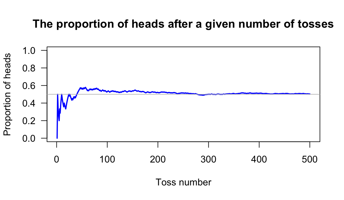

FIGURE 1.4: A simulation of tossing a fair coin \(500\) times. The probability of getting a head is computed from the data after each toss.

Using the empirical approach shows why probabilities are between 0 and 1 (inclusive), since the proportions \(m/n\) are always between 0 and 1 (inclusive).

1.7.2 Classical approach

The classical approach requires being able to define a sample space containing a set of equally-likely outcomes. In practice, this is only true for trivial random processes, like tossing coins, rolling dice, and dealing cards. In the classical approach, random process with \(n\) equally-likely outcomes have all outcomes assigned the probability \(1/n\).

For the calculation of probabilities for events in a sample space with a finite (or countably infinite) number of elements, sometimes sample points can be described so that we have equally-likely outcomes (and hence the classical approach to the assignment of probabilities is appropriate).

Example 1.16 (Tossing dice) When a standard die is tossed, the sample space comprises six equally-likely outcomes: \(S = \{ {1},{2},{3},{4},{5},{6}\}\). The probability of rolling an even number can be computed by counting those outcomes in the sample space that are even (i.e., three events), and dividing by the total number of outcome in the sample space (six events). The probability is \(3/6 = 0.5\).

Associating probabilities with events in this situation is essentially counting sample points. Example 1.16 is a simple demonstration of the principle which we now formalise.

Theorem 1.1 (Equally-likely events) Suppose that a sample space \(S\) consists of \(k\) equally likely elementary events \(E_1\), \(E_2\), \(\ldots\), \(E_k\), and event \(A = \{ E_1, E_2, \ldots, E_r\}\) where \((r\leq k)\). Then \[ \Pr(A) = \frac{r}{k}. \]

This method of calculating the probability of an event is sometimes called the sample-point method. Take care: errors are frequently made by failing to list all the sample points in \(S\).

Methods of counting the points in a sample space with a finite (or countably infinite) number of elements are discussed in Sect. 1.11.4.

Example 1.17 (Lotto) In a game of Oz Lotto, seven numbered balls are drawn from balls numbered 1 to 47. The goal is to correctly pick the seven numbers that will be drawn (without replacing the balls) at random.

There is no reason to suspect that any one number should be more or less likely to occur than any other number. Any set of seven numbers is just a likely to occur as any other set of seven numbers. That is, \[ \{2, 3, 4, 5, 6, 7, 8\} \] is just as likely to be the chosen seven winning numbers as \[ \{4, 15, 23, 30, 33, 39, 45 \}. \]

Listing the sample space is difficult as the number of options is very large for selecting seven numbers from 47.

1.7.3 Subjective approach

‘Subjective’ probabilities are estimated after identifying the information that may influence the probability, and then evaluating and combining this information. You use this method when someone asks you about your team’s chance of winning on the weekend.

The final (subjective) probability may, for example, be computed using mathematical models that use the relevant information. When different people or systems identify different information as relevant, and combine them differently, different subjective probabilities eventuate.

Some examples include:

• What is the chance that an investment will return a positive yield next year?
• How likely is it that Auckland will have above average rainfall next year?

Example 1.18 (Subjective probability) What is the likelihood of rain in Charleville (a town in western Queensland) during April? Many farmers could give a subjective estimate of the probability based on their experience and the conditions on their farm.

Using the classical approach to determine the probability is not possible. While two outcomes are possible—it will rain, or it will not rain—these are almost certainly not equally likely.

A relative frequency approach could be adopted. Data from the Bureau of Meterology, from 1942 to 2022 (81 years), shows rain fell in 71 years during April. An approximation to the probability is therefore \(71 / 81 = 0.877\), or \(87.7\)%. This approach does not take into account current climatic or weather conditions, that can change every year.

1.7.4 Axiomatic approach

An axiom is a self-evident truth that does not require proof, or cannot be proven. Perhaps surprisingly, only three axioms of probability are needed, from which all other results in probability can be proven.

Definition 1.11 (Three axioms of probability) Consider a sample space \(S\) for a random process. For every event \(A\) (a subset of \(S\)), a number \(\Pr(A)\) can be assigned which is called the probability of event \(A\).

The three axioms of probability are:

1. Non-negativity: \(\Pr(A) \ge 0\).
2. Exhaustive: \(\Pr(S) = 1\).
3. Additivity: If \(A_1\), \(A_2\), \(\dots\) form a sequence of pairwise mutually exclusive events in \(S\), then \[ \Pr(A_1 \cup A_2 \cup A_3 \cup \dots) = \sum_{i = 1}^\infty \Pr(A_i). \]

In simple terms, these three axioms state:

1. Probabilities are never negative numbers.
2. The probability that something and only something listed in the sample space will occur is one. (Recall that the sample space lists every possible outcome.)
3. For mutually exclusive events, the probability of the union of events is the sum of the individual probabilities.

While these axioms can sometimes help to assign probabilities, their main purpose is to formally define the rules that apply to probabilities. These axioms of probability can be used to develop all other probability formulae.

Example 1.19 (Using the axioms) Consider proving that \(\Pr(\emptyset) = 0\). While this may appear ‘obvious’, it is not one of the three axioms.

By definition, the empty set \(\emptyset\) contain no points; hence \(\emptyset \cup A = A\) for any event \(A\). Also, \(\emptyset\cap A = \emptyset\), as \(\emptyset\) and \(A\) are mutually exclusive (that is, they have no elements in common). Hence, by the third axiom
\[\begin{equation} \Pr(\emptyset\cup A) = \Pr(\emptyset) + \Pr(A). \tag{1.1} \end{equation}\] But since \(\emptyset \cup A = A\), then \(\Pr(\emptyset \cup A) = \Pr(A)\), and so \(\Pr(A) = \Pr(\emptyset) + \Pr(A)\) from Eq. (1.1). Hence \(\Pr(\emptyset) = 0\).

While this result may have seemed obvious, all probability formulae can be developed just from assuming the three axioms of probability.

1.8 Assigning probabilities: continuous events

Continuous events refer to sets that do not have distinct outcomes to which probabilities can be assigned. Instead, probabilities are assigned to intervals of the sample space, and these probabilities are described using a real-valued probability function, say \(f_X(x)\).

In the discrete case, the probability of observing an element of the sample space must sum to one; for a continuous sample space, the equivalent statement involves integration over the sample space rather than summations.

Since the three axioms of probability still apply, we have:

1. Non-negativity: integration over any region of the sample space must never produce a negative value: \(f_X(x) \ge 0\) for all values of \(x\).
2. Exhaustive: Over the whole sample space, the probability function must integrate to one: \[ \int_S f(x)\,dx = 1. \]
3. Additivity: The probability of the union of any non-overlapping regions is the sum of the individual regions: \[ \int_{A_1} f(x)\, dx + \int_{A_2} f(x)\, dx = \int_{A_1 \cup A_2} f(x)\, dx. \]

Using these axioms implies a probability function for some event \(A\) is defined on the continuous sample space \(S\) as \[ \Pr(X\in A) = \int_{A(x)} f_X(x)\, dx. \]

The probability function \(f_X(x)\) does not give the probability of observing the value \(X = x\). Because the sample space has an infinite number of elements, the probability of observing any single point is zero. Instead, probabilities are computed for intervals.

This implies that \(f_X(x) > 1\) may be true for some values of \(x\), provided the total area over the sample space is one.

Example 1.20 (Assigning probabilities) Suppose I throw a cricket ball \(100\) times, and record the distance thrown. About \(10\)% of the time, the distance is at least \(50\)m but less than \(60\)m; \(20\)% of the time at least \(40\)m; \(50\)% of the time at least \(30\)m; and \(100\)% of the time at least \(20\)m.

With this information we have some idea of the probabilities that my throw goes for certain ranges of distance (Fig. 1.5, left panel).

For these areas to represent probabilities, though, the total area must sum to one. Each rectangle has a width of 10m, and we can define the vertical-axis steps as shown as a distance of \(k\) apart.

The area of each rectangle is easily found, and must sum to one; hence: \[ (10\times 5k) + (10\times 3k) + (10\times k) + (10\times k) = 1, \] so that \(k = 1/100\). With this information, we can create a rough (and coarse) probability model (Fig. 1.5, right panel).

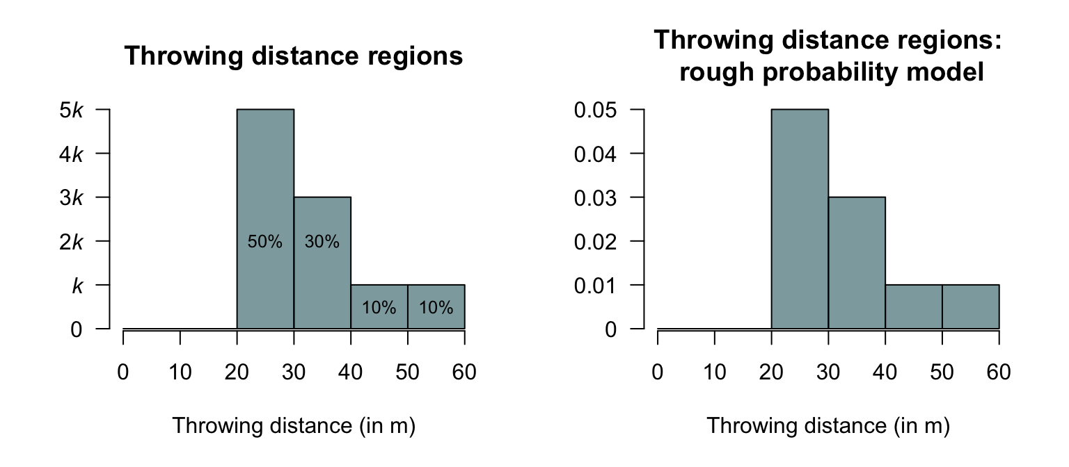
FIGURE 1.5: A rough probability model for throwing distance

1.9 Rules of probability

Many useful results can be deduced from the three axioms which allow probabilities to be computed in more complicated situations.

Theorem 1.2 (Complementary rule of probability) For any event \(A\), the probability of ‘not \(A\)’ is \[ \Pr(\overline{A}) = 1 - \Pr(A). \]

Proof. By the definition of the complement of an event, \(\overline{A}\) and \(A\) are mutually exclusive. Hence, by the third axiom, \(\Pr(\overline{A} \cup A) = \Pr(\overline{A}) + \Pr(A)\).

As \(\overline{A}\cup A = S\) (by definition of the complement) and \(\Pr(S) = 1\) (Axiom 2), then \(1 = \Pr(\overline{A}) + \Pr(A)\), and the result follows.

Theorem 1.3 (Addition rule of probability) For any two events \(A\) and \(B\), the probability of either \(A\) or \(B\) occurring is \[ \Pr(A\cup B) = \Pr(A) + \Pr(B) - \Pr(A\cap B). \]

Proof. Exercise.

If the two events are mutually exclusive, we have a corollary of Theorem 1.3.

Corollary 1.1 If the two events \(A\) and \(B\) are mutually exclusive, then the probability of either \(A\) or \(B\) is \[ \Pr(A\cup B) = \Pr(A) + \Pr(B). \]

Proof. Exercise.

Some other important results that follow from the axioms are the following.

• \(0 \leq \Pr(A) \leq 1\).
• For events \(A\) and \(B\), \(\Pr(A\cup B) \leq \Pr(A) + \Pr(B)\).
• For events \(A\) and \(B\), if \(A\subseteq B\) then \(\Pr(B\cap \overline{A}) = \Pr(B) - \Pr(A)\).
• For events \(A\) and \(B\), if \(A\subseteq B\) then \(\Pr(A) \leq \Pr(B)\).

Proof. Exercises.

1.10 Conditional probability and independence

1.10.1 Conditional probability

Assume that a sample space \(S\) for the random process has been constructed, an event \(A\) has been identified, and its probability, \(\Pr(A)\), has been determined. We then receive additional information that some event \(B\) has occurred. Possibly, this new information can change the value of \(\Pr(A)\).

We now need to determine the probability that \(A\) will occur, given that we know the information provided by event \(B\). We call this probability the conditional probability of \(A\) given \(B\), denoted by \(\Pr(A \mid B)\).

Example 1.21 (Conditional probability) Suppose I roll a die. Define event \(A\) as ‘rolling a 6’. Then, you would compute \(\Pr(A) = 1/6\) (using the classical approach).

However, suppose I provide you with extra information: I tell you that event \(B\) has already occurred, where \(B\) is the event ‘the number rolled is even’.

With this extra information, only three numbers could possibly have been rolled; the reduced sample space is \[ S^* = \{2, 4, 6 \}. \] All of these outcomes are equally likely. However, the probability that the number is a six is now \(\Pr(A\mid B) = 1/3\).

Knowing the extra information in event \(B\) has changed the calculation of \(\Pr(A)\).

Example 1.22 (Planes) Consider these two events: \[\begin{align*} D:&\quad \text{A person dies};\\ F:&\quad \text{A person falls from an airborne plane with no parachute}. \end{align*}\] Consider the probability \(\Pr(D \mid F)\). If you are told that someone falls out of an airborne plane with no parachute, the probability that they die is very high.

Then, consider the probability \(\Pr(F\mid D)\). If you are told that some has died, the cause is very unlikely to be a fall from an airborne plane.

Thus, the first probability is very close to one, and the second is very close to zero.

Two methods exist for computing conditional probability: first principles, or a formal definition of \(\Pr(A \mid B)\). Using first principles, consider the original sample space \(S\), remove the sample points inconsistent with the new information that \(B\) has provided, form a new sample space, say \(S^*\), and recompute the probability of event \(A\) relative to \(S^*\). \(S^*\) is called the reduced sample space.

This method is appropriate when the number of outcomes is relatively small. The following formal definition applies more generally.

Definition 1.12 (Conditional probability) Let \(A\) and \(B\) be events in \(S\) with \(\Pr(B) > 0\). Then \[ \Pr(A \mid B) = \frac{\Pr(A\cap B)}{\Pr(B)}. \]

The definition automatically takes care of the sample space reduction noted earlier.

Example 1.23 (Rainfall) Consider again the rainfall at Charleville in April (Example 1.18). Define \(L\) as the event ‘receiving more than \(30\) mm in April’, and \(R\) as the event ‘receiving any rainfall in April’. Event \(L\) occurs 24 times in the 81 years of data, while event \(R\) occurs 71 times.

Using the relative frequency approach with the Bureau of Meteorology data, the probability of obtaining more than \(30\) mm in April is: \[ \Pr(L) = \frac{24}{81} = 0.296. \] However, the conditional probability of receiving more than \(30\) mm, given that some rainfall was recorded, is: \[ \Pr(L \mid R) = \frac{\Pr(L \cap R)}{\Pr(R)} = \frac{\Pr(L)}{\Pr(R)} = \frac{0.2963}{0.8765} = 0.338. \] If we know rain has fallen, the probability that the amount was greater than \(30\) mm is 0.338. Without this prior knowledge, the probability is 0.296.

Example 1.24 (Conditional probability) Soud et al. (2009) discusses the response of students to a mumps outbreaks in Kansas in 2006. Students were asked to isolate; Table 1.2 shows the behaviour of male and female student in the studied sample.

For females, the probability of complying with the isolation request is: \[ \Pr(\text{Compiled} \mid \text{Females}) = 63/84 = 0.75. \] For males, the probability of complying with the isolation request is \[ \Pr(\text{Compiled} \mid \text{Males}) = 36/48 = 0.75. \]

Whether we look at only females or only males, the probability of selecting a student in the sample that complied with the isolation request is the same: \(0.75\). Also, the non-conditional probability that a student isolated (ignoring their sex) is: \[ \Pr(\text{Student isolated}) = \frac{99}{132} = 0.75. \]

TABLE 1.2: Students response to isolation request at a Kansas university

	Complied with isolation	Did not comply with isolation	TOTAL
Females	63	21	84
Males	36	12	48

1.10.2 Multiplication rule

A consequence of Def. 1.12 is the following theorem.

Theorem 1.4 (Multiplication rule for probabilities) For any events \(A\) and \(B\), the probability of \(A\) and \(B\) is \[\begin{align*} \Pr(A\cap B) &= \Pr(A) \Pr(B \mid A)\\ &= \Pr(B) \Pr(A \mid B). \end{align*}\]

This rule can be generalised to any number of events. For example, for three events \(A\), \(B\), \(C\), \[ \Pr(A\cap B\cap C) = \Pr(A)\Pr(B\mid A)\Pr(C\mid A\cap B). \]

1.10.3 Independent events

The important idea of independence can now be defined.

Definition 1.13 (Independence) Two events \(A\) and \(B\) are independent if and only if \[ \Pr(A\cap B) = \Pr(A)\Pr(B). \] Otherwise the events dependent (or not independent).

Proof. Exercise.

Provided \(\Pr(B) > 0\), Defs. 1.12 and 1.13 show that \(A\) and \(B\) are independent if, and only if, \(\Pr(A \mid B) = \Pr(A)\). This statement of independence makes sense: \(\Pr(A \mid B)\) is the probability of \(A\) occurring if \(B\) has already occurred, while \(\Pr(A)\) is the probability that \(A\) occurs without any knowledge of whether \(B\) has occurred or not. If these are equal, then \(B\) has occurring has made no difference to the probability that \(A\) occurs, which is what independence means.

Example 1.25 In Example 1.24, the probability of males isolating was the same as the probability of females isolating. The sex of the student is independent of whether they isolate. That is, whether we look at females or males, the probability that they isolated is the same.

The idea of independence can be generalised to more than two events. For three events, the following definition of mutual independence applies, which naturally extends to any number of events.

Definition 1.14 (Mutual independence) Three events \(A\), \(B\) and \(C\) are mutually independent if, and only if, \[\begin{align*} \Pr(A\cap B) & = \Pr(A)\Pr(B).\\ \Pr(A\cap C) & = \Pr(A)\Pr(C).\\ \Pr(B\cap C) & = \Pr(B)\Pr(C).\\ \Pr(A\cap B\cap C) & = \Pr(A) \Pr(B) \Pr(C). \end{align*}\]

Three events can be pairwise independent in the sense of Def. 1.13, but not be mutually independent.

The following theorem concerning independent events is sometimes useful.

Theorem 1.5 (Independent events) If \(A\) and \(B\) are independent events, then

• \(A\) and \(\overline{B}\) are independent.
• \(\overline{A}\) and \(B\) are independent.
• \(\overline{A}\) and \(\overline{B}\) are independent.

Proof. Exercise.

1.10.4 Independence and mutually exclusive events {IndependentEvents]}

Mutually exclusive and independent events sometimes get confused.

The simple events defined by the outcomes in a sample space are mutually exclusive, since only one can occur in any realisation of the random process. Mutually exclusive events have no common outcomes: for example, both passing and failing this course is not possible in the one semester. Obtaining one excludes the possibility of the other… so whether one occurs depends on whether the other has occurred.

In contrast, if two events are independent, then whether or not one occurs does not affect the chance of the other happening. If event \(A\) can occur, then \(B\) happening will not influence the chance of \(A\) happening if they are independent, so it does not exclude the possibility of the other occurring.

Confusion between mutual exclusiveness and independence arises sometimes because the sample space is not clearly identified.

Consider a random process involving tossing two coins at the same time. The sample space is \[ S_2 = \{(HH), (HT), (TH), (TT)\} \] and these outcomes are mutually exclusive, each with probability \(1/4\) (using the classical approach). For example, \(\Pr\big( (HH) \big) = 1/4\).

An alternative view of this random process is to think of repeating the process of tossing a coin once. For one toss of a coin, the sample space \[ S_1 = \{ H, T \} \] and \(\Pr(H) = 1/2\) is the probability of getting a head on the first toss. This is also the probability of getting a head on the second toss.

The events ‘getting a head on the first toss’ and ‘getting a head on the second toss’ are not mutually exclusive, because both events can occur together: the event \((HH)\) is an outcome in \(S_2\). Whether or not the outcomes \((HH)\) occurred simultaneously, because the two coins were tossed at the one time, or sequentially, in that one coin was tossed twice, is irrelevant.

Our interest is in the joint outcomes from two tosses. The event ‘getting a head on the “first” toss’ is: \[ E_1 = \{ (HH), (HT) \} \] and ‘getting a head on the “second” toss’ is \[ E_2 = \{ (HH), (TH) \}, \] where \(E_1\) and \(E_2\) are events defined on \(S_2\). This makes it clear that \(E_1\) and \(E_2\) are not mutually exclusive because \(E_1\cap E_2 \ne \emptyset\).

The two events \(E_1\) and \(E_2\) are independent because, whether or not a head occurs on one of the tosses, the probability of a head occurring on the other is still \(1/2\). Seeing that the events are independent provides another way of calculating the probability of the two heads occurring ‘together’: \(1/2\times 1/2 = 1/4\), since the probabilities of independent events can be multiplied

Example 1.26 (Mendell's peas) Mendel (1886) conducted famous experiments in genetics. In one study, Mendel crossed a pure line of round yellow peas with a pure line of wrinkled green peas. Table 1.3 shows what happened in the second generation. For example, \(\Pr(\text{round peas}) = 0.7608\). Biologically, about \(75\)% of peas are expected to be round; the data appear reasonably sound in this respect.

Is the type of pea (rounded or wrinkled) independent of the colour? That is, if the pea is rounded, does it impact the colour of the pea?

Independence can be evaluated using the formula is \(\Pr(\text{round} \mid \text{yellow}) = \Pr(\text{round})\). In other words, the fact that the pea is yellow does not affect that probability that the pea is rounded. From Table 1.3: \[\begin{align*} \Pr(\text{rounded}) &= 0.5665 + 0.1942 = 0.7608,\\ \Pr(\text{round} \mid \text{yellow}) &= 0.5665/(0.5665 + 0.1817) = 0.757. \end{align*}\]

These two probabilities are very close. The data in the table are just a sample (from the population of all peas), so assuming the colour and shape of the peas are independent is reasonable.

TABLE 1.3: The second generation results from Mendel’s experiment, crossing a pure line of round yellow peas with a pure line of wrinkled green peas

	Yellow	Green
Rounded	0.5665	0.1942
Wrinkled	0.1817	0.0576

1.10.5 Partitioning the sample space

The concepts introduced in this section allow us to determine the probability of an event using the event-decomposition approach, which we now discuss.

Definition 1.15 (Partitioning) The events \(B_1, B_2, \ldots , B_k\) are said to represent a partition of the sample space \(S\) if

1. They are mutually exclusive: \(B_i \cap B_j = \emptyset\) for all \(i \neq j\).
2. The events are exhaustive: \(B_1 \cup B_2 \cup \ldots \cup B_k = S\).
3. The events have a non-zero probability of occurring: \(\Pr(B_i) > 0\) for all \(i\).

The implication is that when the random process is performed, one and only one of the events \(B_i\) (\(i = 1, \ldots, k)\) occurs. We use this concept in the following theorem.

Theorem 1.6 (Theorem of total probability) Let \(A\) be an event in \(S\) and \(\{B_1, B_2, \ldots , B_k\}\) a partition of \(S\). Then \[\begin{align*} \Pr(A) &= \Pr(A \mid B_1) \Pr(B_1) + \Pr(A \mid B_2)\Pr(B_2) + \ldots \\ & \qquad {} + \Pr(A \mid B_k)\Pr(B_k). \end{align*}\]

Proof. The proof follows from writing \(A = (A\cap B_1) \cup (A\cap B_2) \cup \ldots \cup (A\cap B_k)\), where the events on the RHS are mutually exclusive. The third axiom of probability together with the multiplication rule yield the result.

Example 1.27 (Theorem of total probability) Consider event \(A\): ‘rolling an even number on a die’, and also define the events \[ B_i:\quad\text{The number $i$ is rolled on a die} \] where \(i = 1, 2, \dots 6\). The events \(B_i\) represent a partition of the sample space.

Then, using the Theorem of total probability (Sect. 1.6):
\[\begin{align*} \Pr(A) &= \Pr(A \mid B_1)\times \Pr(B_1)\quad + \quad\Pr(A \mid B_2)\times \Pr(B_2) \quad+ {}\\ &\quad \Pr(A \mid B_3)\times \Pr(B_3)\quad + \quad\Pr(A\mid B_4)\times \Pr(B_4) \quad+ {} \\ &\quad \Pr(A \mid B_5)\times \Pr(B_5)\quad + \quad\Pr(A\mid B_6)\times \Pr(B_6)\\ &= \left(0\times \frac{1}{6}\right) + \left(1\times \frac{1}{6}\right) + {} \\ &\quad \left(0\times \frac{1}{6}\right) + \left(1\times \frac{1}{6}\right) + {}\\ &\quad \left(0\times \frac{1}{6}\right) + \left(1\times \frac{1}{6}\right) = \frac{1}{2}. \end{align*}\] This the same answer obtained using the classical approach.

1.10.6 Bayes’ theorem

If an event is known to have occurred (i.e., non-zero probability), and the sample space is partitioned, a result known as Bayes’ theorem enables us to determine the probabilities associated with each of the partitioned events.

Theorem 1.7 (Bayes' theorem) Let \(A\) be an event in \(S\) such that \(\Pr(A) > 0\), and \(\{ B_1, B_2, \ldots , B_k\}\) is a partition of \(S\). Then \[ \Pr(B_i \mid A) = \frac{\Pr(B_i) \Pr(A \mid B_i)} {\displaystyle \sum_{j = 1}^k \Pr(B_j)\Pr(A \mid B_j)} \] for \(i = 1, 2, \dots, k\).

Proof. This is a direct application of Def. 1.12, the multiplication rule and Theorem 1.6.

Notice that the right-side includes conditional probabilities of the form \(\Pr(A\mid B_i)\), while the left-side contains the probability \(\Pr(B_i\mid A)\). In effect, the theorem takes a conditional probability and can ‘reverse’ the conditioning.

Bayes’ theorem has many uses, as it uses conditional probabilities that are easy to find or estimate to compute a conditional probability that is not easy to find or estimate. The theorem is the basis of a branch of statistics known as Bayesian statistics which involves using pre-existing evidence in drawing conclusions from data.

Example 1.28 (Breast cancer) The success of mammograms for detecting breast cancer has been well documented (White, Urban, and Taylor 1993). Mammograms are generally conducted on women over \(40\), though breast cancer rarely occurs in women under \(40\).

We can define two events of interest: \[\begin{align*} C:&\quad \text{The woman has breast cancer; and}\\ D:&\quad \text{The mammogram returns a positive test result.} \end{align*}\] As with any diagnostic tool, a mammogram is not perfect. Sensitivity and specificity are used to describe the accuracy of a test:

• Sensitivity is the probability of a true positive test result: the probability of a positive test result for people with the disease. This is \(\Pr(D \mid C)\).
• Specificity is the probability of a true negative test result: the probability of a negative test for people without the disease. This is \(\Pr(\overline{D} \mid \overline{C})\).

Clearly, we would like both these probabilities to be a high as possible. For mammograms (Houssami et al. 2003), the sensitivity is estimated as about \(0.75\) and the specificity as about \(0.90\). We can write:

• \(\Pr(D \mid C ) = 0.75\) (and so \(\Pr(\overline{D} \mid C) = 0.25\));
• \(\Pr(\overline{D} \mid \overline{C}) = 0.90\) (and so \(\Pr(D \mid \overline{C}) = 0.10\)).

Furthermore, about 2% of women under 40 will get breast cancer (Houssami et al. 2003); that is, \(\Pr(C) = 0.02\) (and hence \(\Pr(\overline{C}) = 0.98\)).

For this study, the probabilities \(\Pr(D\mid C)\) are easy to find: women who are known to have breast cancer have a mammogram, and we record whether the result is positive or negative.

But consider a woman under \(40\) who gets a mammogram. When the results are returned, her interest is whether they have breast cancer, given the test results; for example \(\Pr(C \mid D)\). In other words: If the test returns a positive result, what is the probability that she actually has breast cancer?

That is, we would like to take probabilities like \(\Pr(D\mid C)\), that can be found readily, and determine \(\Pr(C \mid D)\), which is of interest in practice. Using Bayes’ Theorem: \[\begin{align*} \Pr(C \mid D) &= \frac{\Pr(C) \times \Pr(D \mid C)} {\Pr(C)\times \Pr(D \mid C) + \Pr(\overline{C})\times \Pr(D \mid \overline{C}) }\\ &= \frac{0.02 \times 0.75} {(0.02\times 0.75) + (0.98\times 0.10)}\\ &= \frac{0.015}{0.015 + 0.098} = 0.1327. \end{align*}\] Consider what this says: Given that a mammogram returns a positive test (for a woman under \(40\)), the probability that the woman really has breast cancer is only about \(6\)%… This partly explains why mammograms for women under \(40\) are not commonplace: most women who return a positive test result actually do not have breast cancer.

The reason for this surprising result is explained in Example 1.29.

1.11 Computing probabilities

Different schemes can be used to help compute probabilities, such as tree diagrams, tables, Venn diagrams and counting. Typically, multiple methods may be applied to a given situation, but one method is often easier to apply.

1.11.1 Tree diagrams

Tree diagrams are useful when a random process can be seen, or thought of, as occurring in steps or stages. The branches in the ‘second stage’ are conditional probabilities, conditional on the branch of the first step. Of course, the ideas extend to multiple steps.

Example 1.29 (Breast cancer) Consider using a tree diagram to describe the breast cancer information from Example 1.28 (Fig. 1.6). By following each ‘branch’ of the tree, we can compute, for example: \[ \Pr(C \cap D) = \Pr(C)\times \Pr(D\mid C) = 0.02 \times 0.75 = 0.015; \] that is, the probability that a woman has a positive test and breast cancer is about \(0.015\). But compare: \[ \Pr(\overline{C} \cap D) = \Pr(\overline{C})\times \Pr(D\mid \overline{C}) = 0.98 \times 0.10 = 0.098; \] that is, the probability that a woman has a positive test and no breast cancer (that is, a false positive) is about \(0.098\).

This explains the surprisingly result in Example 1.28: because breast cancer is so uncommon in younger women, the false positives (\(0.098\)) overwhelm the true positives (\(0.015\)).

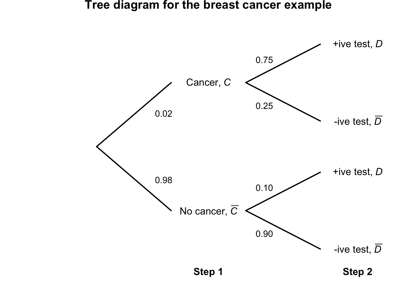
FIGURE 1.6: Tree diagram for the breast-cancer example

1.11.2 Tables

With two variables of interest, tables may be a convenient way of summarizing the information. Although tables can be used to represent random processes using conditional probabilities, usually tables are used to represent the whole sample space.

Example 1.30 (Breast cancer) The breast-cancer data in Example 1.28 can also be compiled into a table giving the four outcomes in the sample space (Table 1.4).

TABLE 1.4: The probabilities from the breast cancer example

	+ive test	-ive test	Total
Has breast cancer	\(0.75 \times 0.02 = 0.015\)	\(0.25 \times 0.02 = 0.005\)	0.02
Does not have breast cancer	\(0.10 \times 0.98 = 0.098\)	\(0.90 \times 0.98 = 0.882\)	0.98

1.11.3 Venn diagrams

Venn diagrams can be useful when there are two events, sometimes three, but become unworkable for more than three. Often, tables can be used to better represent situations shown in Venn diagrams.

Example 1.31 (Breast cancer) Consider again the breast cancer data (Example 1.28, where the events \(C\) and \(D\) were defined earlier). A Venn diagram could be constructed to show the sample space (Fig. 1.7).

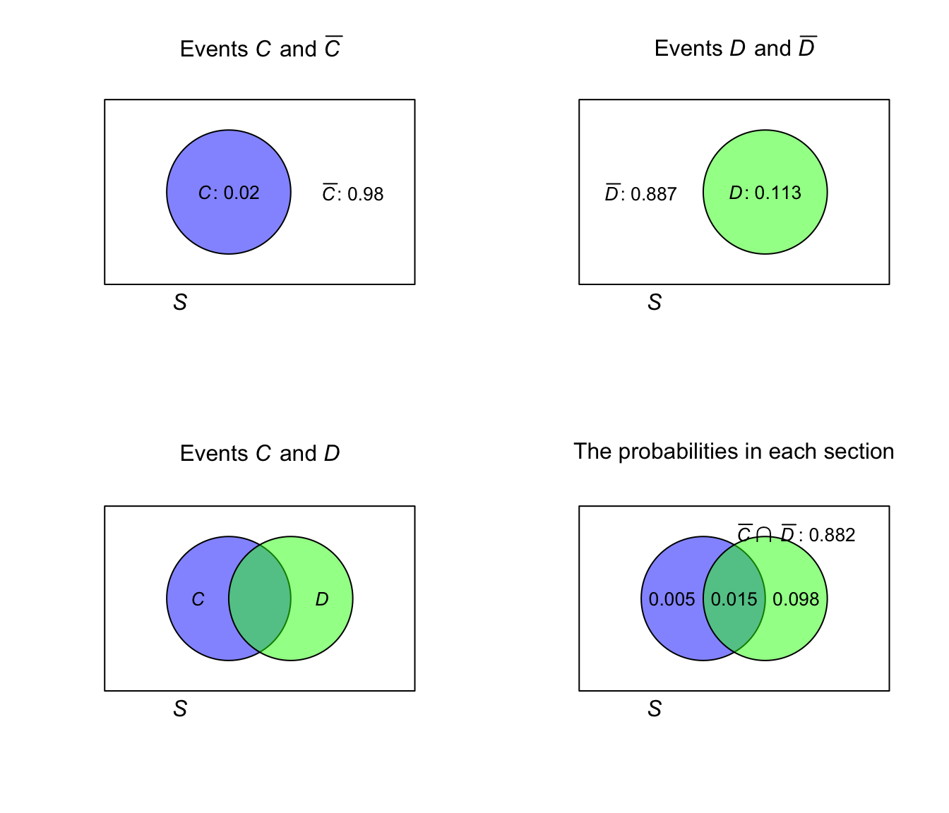
FIGURE 1.7: The Venn diagram for the breast cancer example

1.11.4 Counting sample spaces

Sometimes the most convenient way to compute probabilities is to list the sample space. This only works for sample spaces with a small number of discrete elements, and works best when each of the outcomes in the sample space are equally likely.

Example 1.32 (Rolling two dice) Consider rolling two standard dice and noting the sum of the numbers shown. The sample space is listed in Table 1.5. Then, for example, \(\Pr(\text{sum is 7}) = 6/36\) is found by counting the equally-likely outcomes that sum to seven.

TABLE 1.5: The sum of rolling two dice

	Die 2: 1	Die 2: 2	Die 2: 3	Die 2: 4	Die 2: 5	Die 2: 6
Die 1: 1	2	3	4	5	6	7
Die 1: 2	3	4	5	6	7	8
Die 1: 3	4	5	6	7	8	9
Die 1: 4	5	6	7	8	9	10
Die 1: 5	6	7	8	9	10	11
Die 1: 6	7	8	9	10	11	12

The number of elements in a set is often large, and a complete enumeration of the set is unnecessary if all we want to do is to count the number of elements in the set. When the number of elements in the sample space is large, principles and formulae exist which aid counting, some of which are described in the following sections.

1.11.5 Multiplication principle

If we have \(m\) ways to perform act \(A\) and if, for each of these, there are \(n\) ways to perform act \(B\), then there are \(m\times n\) ways to perform the acts \(A\) and \(B\). This is called the multiplication principle.

Definition 1.16 (Multiplication principle) With \(m\) elements \(a_1, a_2, \ldots , a_m\) and \(n\) elements \(b_1, b_2, \ldots, b_n\) then \(mn\) pairs can be made containing one element from each group.

The principle can be extended to any number of sets. For example: For three sets of elements \(a_1, a_2, \ldots , a_m\), \(b_1, b_2, \ldots , b_n\) and \(c_1, c_2, \ldots , c_p\), the number of distinct triplets containing one element from each set is \(mnp\).

Example 1.33 (Multiplication principle) Suppose a restaurants offers five main courses and three desserts. If a ‘meal’ consists of one main plus one dessert, then \(5\times 3 = 15\) meal combinations are possible.

1.11.6 Permutations

Another important counting problem deals with different permutations of a finite set. The word permutation in this context means an ordering of the set: selecting elements when the selection order is important.

1.11.6.1 Selecting without replacement

Suppose a set has \(n\) elements. To order these, the first element of the ordering must initially be chosen, which can be done in \(n\) different ways. The second element must then be chosen, which can be done in \((n - 1)\) ways (since it cannot be the same as the first). There are then \((n - 2)\) ways for the third, and so on.

We find (using the multiplication principle) that there are \(n(n - 1)(n - 2)\ldots 2 \times 1\) different ways to order the \(n\) elements. This is denoted by \(n!\) and called ‘\(n\)-factorial’: \[ n! = n(n - 1)(n - 2) \ldots (2)(1) \] where \(n\geq 1\), and we define \(0! = 1\).

In some cases, the number of ways in which only the first \(r\) elements of an ordering may be chosen is needed.

For this problem, the first element in the ordering may be chosen in \(n\) different ways, the second in \((n - 1)\) ways, the third in \((n - 2)\) ways, and so on… down to the \(rth\), which may be chosen in \((n - r + 1)\) ways.

This number is denoted by \(^nP_r\), and we write
\[\begin{equation} ^nP_r = n(n - 1)(n - 2)\ldots (n - r + 1) = \frac{n!}{(n - r)!}. \tag{1.2} \end{equation}\] This expression is referred to as the number of permutations of \(r\) elements from a set with \(n\) elements.

Notation for permutations varies. Other notation for permutations include \(nPr\), \(^nP_r\), \(P_n^r\) or \(P(n,r)\).

By definition, \(0! = 1\). With this definition, many formulas (some follow) remain valid for all valid choices of \(n\) and \(r\).

Example 1.34 (Permutations) Suppose a company requires users to select a password of eight characters using only lower-case letters. Since the order of the letters is important in a password, we work with permutations. There are \[ \displaystyle {}^{26}P_8 = \frac{26!}{(26 - 8)!} = 62\,990\,928\,000 \] possible passwords to select.

1.11.6.2 Selecting with replacement

If each item can be re-selected (for example, the item is returned to the larger pool of items), we say that selection is done with replacement.

The number of ordered selections of \(r\) objects chosen from \(n\) with replacement is \(n^r\). The first object can be selected in \(n\) ways, the second can be selected in \(n\) ways, etc., and by the multiplication principle, we have \(n^r\) possible outcomes.

1.11.7 Combinations

In some cases, order is not important when choosing a subset (i.e., when dealing a hand of cards). A combination of \(r\) elements from a set \(S\) is a subset of \(S\) with exactly \(r\) elements.

1.11.7.1 Selecting without replacement

The number of combinations of \(r\) elements from a set with \(n\) distinct elements is denoted by \(^nC_r\). The number of permutations is given by Eq. (1.2), but the number of combinations must be smaller, since many permutations are equivalent to the same combination. In fact, each combination of \(r\) elements can be ordered in \(r!\) different ways, and so gives rise to \(r!\) permutations. Hence, the number of permutations must be \(r!\) times the number of combinations. We have then, \[ ^nC_r = \frac{n(n - 1)\ldots (n - r + 1)}{r!} = \frac{n!}{(n - r)!\,r!} = \frac{^n P_r}{r!}. \]

Notation for combinations varies. Other notation for combinations include \(nCr\), \(^nC_r\), \(C_n^r\), \(\binom{n}{r}\) or \(C(n,r)\).

The difference between permutations and combinations is important! With permutations, the selection order is important, whereas selection order is not important with combinations. In addition, both formulae apply when there is no replacement of the items.

This may help you remember when to use permutations and combinations

• Permutations are used for passwords.
• Combinations are used when dealing cards.

Example 1.35 (Selecting digits) Consider the set of integers \({1, 3, 5, 7}\). Choose two numbers, without replacement; call the first \(a\) and the second \(b\). If we then compute \(a\times b\), then \(^4C_2 = 6\) answers are possible since the selection order is not important (e.g., \(3 \times 7\) gives the same answer as \(7 \times 3\)).

However, if we compute \(a\div b\), then \(^4P_2 = 12\) answers are possible, since the selection order is important (e.g., \(3 \div 7\) gives a different answer than \(7 \div 3\)).

Example 1.36 (Oz Lotto combinations) In Oz Lotto, players select seven numbers from 47, and try to match these with seven randomly selected numbers. The order in which the seven numbers are selected in not important, so combinations (not permutations) are appropriate. That is, winning numbers drawn in the order, as \(\{1, 2, 3, 4, 5, 6, 7\}\) are effectively the same as if they were drawn in the order \(\{7, 2, 1, 3, 4, 6, 5\}\).

The number of options for players to choose from is \[ \binom{47}{7} = \frac{47!}{40!\times 7!} = 62\,891\,499; \] that is, almost \(63\) million combinations are possible.

The probability of picking the correct seven numbers in a single guess is therefore \[ \frac{1}{62\,891\,499} = 1.59\times 10^{-8} = 0.000\,000\,015\,9. \]

In R:

• the number of combinations of n elements k at a time is found using choose(n, k).
• a list of all combinations of n elements, m at a time is given by combn(x, m).
• \(n!\) is given by factorial(n).
• \(\Gamma(x)\) is given by gamma(x).

The binomial expansion \[ (a + b)^n = \sum^{n}_{r = 0} \binom{n}{r} a^r b^{n - r} \] for \(n\) a positive integer, is often referred to as the Binomial Theorem and hence \(\binom{n}{r}\) is referred to as a binomial coefficient. This series, and associated properties, is sometimes useful in counting. Some of the properties of combinations are stated below.

1. \(\binom{n}{r} = \binom{n}{n - r}\), for \(r = 0, 1, \ldots, n\).
2. As a special case of the above, \(\binom{n}{0} = 1 = \binom{n}{n}\).
3. \(\sum_{r = 0}^n \binom{n}{r} = 2^n\).

1.11.7.2 Selecting without replacement

The number of ways \(r\) objects can be chosen from \(n\) with replacement and without regard to order is somewhat more difficult and won’t be attempted here. The number of ways is actually \(\binom{n + r - 1}{r}\).

1.12 Introducing statistical computing

1.12.1 Using R

Computers and computer packages are essential tools in the application of statistics to real problems. In this book, the statistical package R is used, and will be used to illustrate various concepts to help you understand the theory (Example 1.15).

One way in which R can be used is to easily compute probabilities for specific distributions. Also, R can be used to verify (not prove) theoretical results obtained. To do this, a technique called computer simulation can be used.

Simulation can also be used to solve problems for which it may be difficult (or impossible) to obtain a theoretical result. Sometimes these numerical solutions to intractable analytical problems is termed Monte Carlo simulation.

1.12.2 Example: the gameshow (Monty Hall) problem

A game show contestant is told there is a car behind one of three doors, and a goat behind each of the other doors. The contestant is asked to select a door.

The host of the show (who knows where the car is) now opens one of the doors not selected by the contestant, and reveals a goat. The host now gives the contestant the choice of either (a) retaining the door chosen first, or (b) switching and choosing the other (unopened) door. Which of the following is the contestant’s best strategy?

1. Always retain the first choice.
2. Always change and select the other door.
3. Choose either unopened door at random.

What strategy do you think would be best?

Only a brief outline of the method is given here. A more complete solution is given later.

1. Generate a random sequence of length \(1000\) of the digits \(1\), \(2\) and \(3\) to represent which door is hiding the car on each of \(1000\) nights.
2. Generate another such sequence to represent the contestants first choice on each of the \(1000\) nights (assumed chosen at random).
3. The number of times the numbers in the two lists of random numbers do agree represents the number of times the contestant will win if the contestant doesn’t change doors. If the numbers in the two columns don’t agree then the contestant will win only if the contestant decides to change doors.

For the \(1000\) nights simulated, contestants would have won the car \(303\) times if they retained their first choice which means they would have won \(697\) times if they had changed. (Does this agree with your intuition?) This implies (correctly!) that the best strategy is to change. You might like to try doing the simulation for yourself.

The correct theoretical probability of winning if you retain the original door is \(1/3\), but \(2/3\) if you change.) We obtained a reasonable estimate of these probabilities from the simulation: \(303/1000\) and \(697/1000\). These estimates would improve for larger simulation sizes.

set.seed(93671)          # For reproducibility

NumSims <- 1000          # The number of simulations
# Choose the door where the car is hiding:
CarDoor <- sample(1:3,  # Could be behind Door 1, 2 or 3
                  size = NumSims, # Repeat
                  replace = TRUE)
# Choose the contestants initial choice:
FirstChoice <- sample(1:3,        # Could guess Door 1, 2 or 3
                  size = NumSims, # Repeat
                  replace = TRUE)

# Compute the chances of winning the car:
WinByNotSwitching  <- sum( CarDoor == FirstChoice)
WinBySwitching     <- sum( CarDoor != FirstChoice)

c(WinByNotSwitching, WinBySwitching) / NumSims
#> [1] 0.303 0.697

1.13 Exercises

Selected answers appear in Sect. D.1.

Exercise 1.1 Suppose \(\Pr(A) = 0.53\), \(\Pr(B) = 0.24\) and \(\Pr(A\cap B) = 0.11\).

1. Display the situation using a Venn diagram, tree diagram and a table. Which is easier in this situation?
2. Find \(\Pr(A\cup B)\).
3. Find \(\Pr(\overline{A}\cap B)\).
4. Find \(\Pr(\overline{A} \cup \overline{B})\).
5. Find \(\Pr(A \mid B)\).
6. Are events \(A\) and \(B\) independent?

Exercise 1.2 Suppose a box contains \(100\) tickets numbered from \(1\) to \(100\) inclusive. Four tickets are drawn from the box one at a time (without replacement). Find the probability that:

1. all four numbers drawn are odd.
2. exactly two odd numbers are drawn.
3. at least two odd numbers are drawn before drawing the first even number.
4. the sum of the numbers drawn is odd.

Exercise 1.3 Consider the solutions to the general quadratic equation \(y = ax^2 + bx + c = 0\) (where \(a \ne 0\), since then the equation does not define a quadratic). Suppose real values are chosen at random for the constants \(a\), \(b\) and \(c\).

1. Define, using the appropriate notation, the sample space \(S\) for the experiment.
2. Define, using the appropriate notation, the event \(R\): ‘the equation has two equal real roots’.
3. Define, using the appropriate notation, the event \(Z\): ‘the equation has no real roots’.

Exercise 1.4 A courier company is interested in the length of time a certain set of traffic lights is green. The lights are set so that the time between green lights in any one direction is between \(15\) and \(150\) seconds. An employee observes the lights and record the length of time between consecutive green lights.

1. What is the random variable?
2. What is the sample space?
3. Can the classical approach to probability be used to determine the probability that the time between green lights is less than \(90\) seconds? Why or why not?
4. Can the relative frequency approach be used to determine the same probability? If so, how? If not, why not?

Exercise 1.5 Suppose a touring cricket squad consist of fifteen players, from which a team of eleven must be chosen for each game. Suppose a squad consists of seven batters, five bowlers, two all-rounders and one wicketkeeper.

1. Find the number of teams possible if the playing team consists of five batters, four bowlers, one all-rounder and one wicketkeeper.
2. After a game, each member of one playing team shakes hands with each member of the opposing playing team, and each member of both playing teams shakes hands with the two umpires. How many handshakes are there in total at the conclusion of a game?

Exercise 1.6 Researchers (Dexter et al. 2019) observed the behaviour of pedestrians in Brisbane, Queensland, around midday in summer. The researchers found the probability of wearing a hat was \(0.025\) for males, and \(0.060\) for females. Using this information:

1. Construct a tree diagram for the sample space.
2. Construct a table of the sample space.
3. Construct the Venn diagram of the sample space.

Exercise 1.7 A family with six non-driving children, and two driving parents has an eight-seater vehicle.

1. In how many ways can the family be seated in the car (and legally go driving)?
2. Suppose one of the children obtains their driving licence. In how many ways can the family be seated in the car (and legally go driving) now?
3. Two of the children needs car seats, and there are two car seats fixed in the vehicle (i.e., they cannot be moved to different seats). If the two parents are the only drivers, in how many ways can the family be seated in the car (and legally go driving) now?

Exercise 1.8 A group of four people sit down to play Monopoly. The eight tokens are distributed randomly. In how many ways can this be done?

Exercise 1.9 A company password policy is that users must select an eight-letter password comprising lower-case letters (Example 1.34). The company is considering each of the following changes separately:

1. Suppose the policy changes to allow eight-, nine-, or ten-letter passwords of just lower-case letters. How many passwords are possible now?
2. Suppose the policy changes to allow eight-letter passwords comprising lower-case and upper-case letters letters. How many passwords are possible now?
3. Suppose the policy changes to allow eight-letter passwords comprising lower-case, upper-case letters letters and the ten digits \(0\) to \(9\). How many passwords are possible now?
4. Suppose the policy changes to allow eight-letter passwords comprising lower-case, upper-case letters letters and the ten digits \(0\) to \(9\), and each password must have one of each category. How many passwords are possible now?

Exercise 1.10 Many document processors help users match brackets. Bracket matching is an interesting mathematical problem! For instance, the string (()) is syntactically valid, whereas ())( is not, even though both contain two opening and two closing brackets.

1. List all the ways in which two opening and two closing brackets can be written in a way that is syntactically valid.
2. How many ways can three opening and three closing brackets be written in a way that is syntactically valid? List these.
3. In general, the number of ways that \(n\) opening and \(n\) closing brackets can be written that is syntactically valid is given by the Catalan numbers \(C_n\), where: \[ C_{n} = {\frac {1}{n + 1}}\binom{2n}{n}. \] Show that an equivalent expression for \(C_n\) is \(\displaystyle C_n = {\frac {(2n)!}{(n + 1)!\,n!}}\).
4. Show that another equivalent expression for \(C_n\) is \(\displaystyle \binom{2n}{n} - \binom{2n}{n + 1}\) for \(n\geq 0\).
5. Find the first nine Catalan numbers, starting with \(C_0\).

Exercise 1.11 Stirling’s approximation is \[ n!\approx {\sqrt {2\pi n}}\left({\frac {n}{e}}\right)^{n}. \]

1. Compare the values of the actual factorials with the Stirling approximation values for \(n = 1, \dots, 10\). (Use technology!)
2. Plot the relative error in Stirling’s approximation for \(n = 1, \dots, 10\). (Again, use technology!)

Exercise 1.12 In a two-person game, a fair die is thrown in turn by each player. The first player to roll a wins.

1. Find the probability that the first player to throw the die wins.
2. Suppose the player to throw first is selected by the toss of a fair coin. Show that each player has an equal chance of winning.

Exercise 1.13 To get honest answers to sensitive questions, sometimes the randomised response technique is used. For example, suppose the aim is to discover the proportion of students who have used illegal drugs in the past twelve months.

\(N\) cards are prepared, where \(m\) have the statement ‘I have used an illegal drug in the past twelve months’. The remaining \(N - m\) cards have the statement ‘I have not used an illegal drug in the past twelve months’.

Each student in the sample then selects one card at random from the prepared pile of \(N\) cards, and answers ‘True’ or ‘False’ when asked the question ‘Is the statement on the selected card true or false?’ without divulging which statement is on the card. Since the interviewer does not know which card has been presented, the interviewer does not know if the person has used drugs or not from this answer.

Let \(T\) be the probability that a student answers ‘True’, and \(p\) be the probability that a student chosen at random has used an illegal drug. Assume that each student answers the question on the chosen card truthfully.

1. From an understanding of the problem, show that \[ T = (1 - p) + \frac{m}{N}(2p - 1). \]
2. Find an expression for \(p\) in terms of \(T\), \(m\) and \(N\) by rearranging the previous expression.
3. Explain what happens for \(m = 0\), \(m = N\) and \(m = N/2\), and why these make sense in the context of the question.
4. Suppose that, in a sample of 400 students, 175 answer ‘True’. Estimate \(p\) from the expression found above, given that \(N = 100\) and \(m = 25\).

Exercise 1.14 A multiple choice question contains \(m\) possible choices. There is a probability of \(p\) that a candidate chosen at random will know the correct answer. If a candidate does not know the answer, the candidate guesses and is equally likely to select any of the \(m\) choices.

For a randomly selected candidate, what is the probability of the question being answered correctly?

Exercise 1.15 In the 2019/2020 English Premier League (EPL), at full-time the home team had won \(91\) out of \(208\) games, the away team won \(67\), and \(50\) games were drawn. (Data from: https://sports-statistics.com/sports-data/soccer-datasets/)

Define \(W\) as a win, and \(D\) as a draw.

1. Explain the difference between \(\Pr(W)\) and \(\Pr(W \mid \overline{D})\).
2. Compute both probabilities, and comment.

Exercise 1.16 Consider a square of size \(1\times 1\) metre. A random process consists of selecting two points at random in the square.

1. What is the sample space for the distance between the two points?
2. Suppose a grid (lines parallel to the sides) is drawn on the square such that grid lines are equally spaced \(25\) cm apart. Two points are chosen again, but must be on the intersection of the grid lines. Write some R code to generate the sample space for the distance between the two points.

Exercise 1.17 Suppose that \(30\)% of the residents of a certain suburb subscribe to a local newsletter. In addition, \(8\)% of residents belong to a local online group.

1. What percentage of residents could belong to both? Give a range of possible values.
2. Suppose \(6\)% belong to both. Compute:
   1. The probability than a random chosen newsletter subscriber is also a member of the online group.
   2. The probability than a random chosen online member is also a subscriber to the newsletter.

Exercise 1.18 The data in Table 1.6 tabulates information about school children in Queensland in 2019 (Dunn 2023).

1. What is the probability that a randomly chosen student is a First Nations student?
2. What is the probability that a randomly chosen student is in a government school?
3. Is the sex of the student approximately independent of whether the student is a First Nations student, for students in government schools?
4. Is the sex of the student approximately independent of whether the student is a First Nations student, for students in non-government schools?
5. Is whether the student is a First Nations student approximately independent of the type of school, for female students?
6. Is whether the student is a First Nations student approximately independent of the type of school, for male students?
7. Based on the above, what can you conclude from the data?

TABLE 1.6: The number of First Nations and non-First Nations students in various Queensland schools in 2019

	Number First Nations students	Number non-First Nations students
Government schools
Females	2540	21219
Males	2734	22574
Non-government schools
Females	391	9496
Males	362	9963

Exercise 1.19 Two cards are randomly drawn (without replacement) from a \(52\)-card pack.

1. What is the probability the second card is an Ace?
2. What is the probability that the first card is lower in rank (Ace low) than the second?
3. What is the probability that the card ranks are in consecutive order where Ace is low or high and order is irrelevant (e.g., (Jack, Queen), (Queen, Jack), (Ace, Two) or (kKng, Ace))?

Exercise 1.20 An octave contains \(12\) distinct notes: seven white keys and 5 black keys on a piano.

1. How many different eight-note sequences within a single octave can be played using the white keys only?
2. How many different eight-note sequences within a single octave can be played if the white and black keys alternate (starting with either colour)?
3. How many different eight-note sequences within a single octave can be played if the white and black keys alternate and no key is played more than once?

Exercise 1.21 Find \(\Pr(A\cap B)\) if \(\Pr(A) = 0.2\), \(\Pr(B) = 0.4\), and \(\Pr(A\mid B) + \Pr(B \mid A) = 0.375\).

Exercise 1.22 Solve \(12\times {}^7P_k = 7\times {}^6P_{k + 1}\) using:

1. algebra; and then
2. using R to search over all possible values of \(k\).

Exercise 1.23 Solve \(^7 P_{r + 1} = 10 {^7 C _r}\) for \(r\).

Exercise 1.24

1. Show that the probability that, for a group of \(N\) randomly selected individuals, at least two have the same birthday (assuming \(365\) days in a year) can be written as \[ 1 - \left(\frac{365}{365}\right) \times \left(\frac{364}{365}\right) \times \left(\frac{363}{365}\right) \times \dots\times \left(\frac{365 - n + 1}{365}\right). \]
2. Graph the relationship for various values of \(N\), using the above form to compute the probability.
3. What assumptions are necessary? Are these reasonable?

Exercise 1.25 Six numbers are randomly selected without replacement from the numbers \(1, 2, 3,\dots, 45\). Model this process using R to estimate the probability that there are no consecutive numbers amongst the numbers selected. (That is, no sequence like 4, 5 or 33, 34 or 21, 22, 23 appears, once the numbers are sorted smallest to largest.)

Exercise 1.26 Suppose the events \(A\) and \(B\) have probabilities \(\Pr(A) = 0.4\) and \(\Pr(B) = 0.3\), and \(\Pr(A\cup B) = 0.5\). Determine \(\Pr( \overline{A} \cap \overline{B})\). Are \(A\) and \(B\) independent events?

Exercise 1.27 For sets \(A\) and \(B\), show that:

1. \(A\cup (A\cap B) = A\);
2. \(A\cap (A\cup B) = A\).

These are called the absorption laws.

Exercise 1.28 A new cars can be purchased with options:

• Seven different paints colours are available;
• Three different trim levels are available;
• Cars can be purchased with or without a sunroof.

How many possible combinations are possible?

Exercise 1.29 Suppose number plates have three numbers, followed by two letters then another number. How many number plates are possible with this scheme?

Exercise 1.30 In some forms of poker, five cards are dealt to each player, and certain combinations then beat other combinations.

1. What is the probability that the initial five cards include exactly one pair. (This implies not getting a three of a kind or four of a kind.) Explain your reasoning.
2. What is the probability that the initial five cards includes only picture cards (Ace, King, Queen, Jack)?

Exercise 1.31 Prove that \({}^n P_n = {}^nP_{n-1}\).

Exercise 1.32 Without using any technology, compute the value of \(\displaystyle \frac{{}^{25} C_8}{{}^{25} C_6}\).

Exercise 1.33 Define these two sets:
\[\begin{align*} S &= \{\clubsuit, \spadesuit, \heartsuit, \diamondsuit\};\\ D &= \{ 2, 3, \dots, 10, \text{Jack}, \text{Queen}, \text{King}, \text{Ace}\}. \end{align*}\] Then, define set \(C\) as ‘cards in a standard pack’.

Write \(C\) in terms of \(S\) and \(D\) using set notation.

Exercise 1.34 Use set notation to show the relationship between the complex numbers \(\mathbb{C}\) and \(\mathbb{R}\).

Exercise 1.35

1. If \(A_1, A_2, \dots, A_n\) are independent events, prove that \[ \Pr(A_1 \cup A_2 \cup \dots \cup A_n) = 1 - [1 - \Pr(A_1)][1 - \Pr(A_2)] \dots [1 - \Pr(A_n)]. \]
2. Consider two events \(A\) and \(B\) such that \(\Pr(A) = r\) and \(\Pr(B) = s\) with \(r, s > 0\) and \(r + s > 1\). Prove that \[ \Pr(A \mid B) \ge 1 - \left(\frac{1 - r}{s} \right). \]

Exercise 1.36 Consider the diagram in Fig. 1.8. The point \(P\) is randomly placed within the \(1\times 1\) square \(ABCD\).

What is the probability that the angle \(APB\) is greater than \(90^\circ\)?

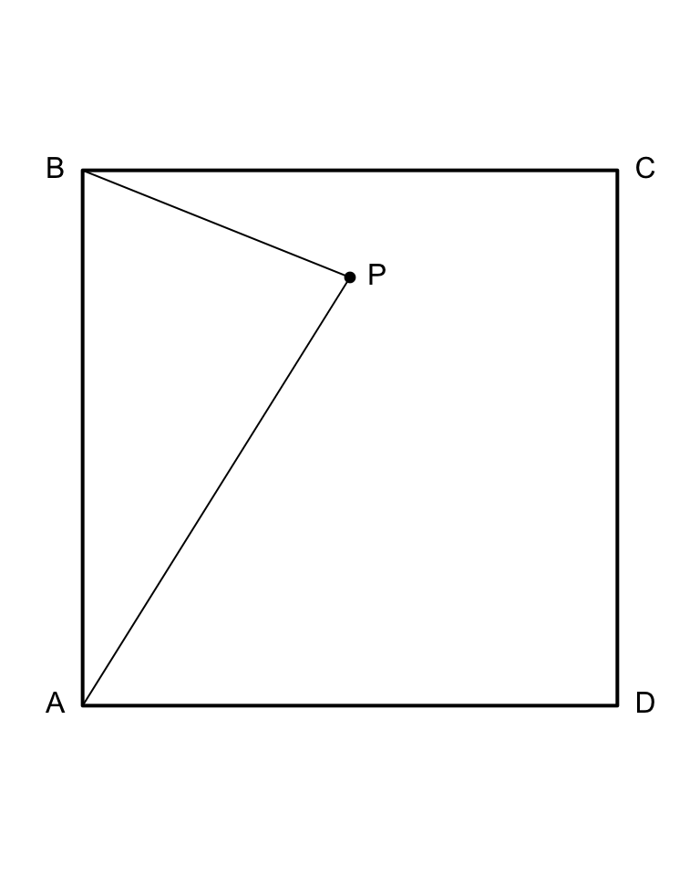
FIGURE 1.8: Point \(P\) is placed randomly in the \(1\times 1\) square \(ABCD\)

---

Peter K. Dunn, 2024: CC BY-NC-SA 4.0