4 Standard discrete distributions

Upon completion of this chapter, you should be able to:

recognise the probability functions and underlying parameters of uniform, Bernoulli, binomial, geometric, negative binomial, Poisson, and hypergeometric random variables.
know the basic properties of the above discrete distributions.
apply these discrete distributions as appropriate to problem solving.

4.1 Introduction

In this chapter, some popular discrete distributions are discussed. Properties such as definitions and applications are considered.

4.2 Discrete uniform distribution

If a discrete random variable $X$ can assume $k$ different and distinct values with equal probability, then $X$ is said to have a discrete uniform distribution. This is one of the simplest discrete distributions.

Definition 4.1 (Discrete uniform distribution) If a random variable $X$ with range space $\{a, a + 1, a + 2, \dots, b\}$, where $a$ and $b$ ($a < b$) are integers, has the pf
\[\begin{equation} p_X(x; a, b) = \frac{1}{b - a + 1}\text{ for $x = a, a + 1, \dots, b$} \tag{4.1} \end{equation}\] then $X$ has a discrete uniform distribution. We write $X\sim U(a, b)$ or $X\sim \text{Unif}(a, b)$.

The notation $p_X(x; a, b)$ means that the probability function for $X$ depends on the parameters $a$ and $b$.

The symbol $\sim$ means ‘is distributed with’; hence, ‘$X\sim U(a, b)$’ means ‘$X$ is distributed with a discrete uniform distribution with parameters $a$ and $b$’.

A plot of the probability function for a discrete uniform distribution is shown in Fig. 4.1.

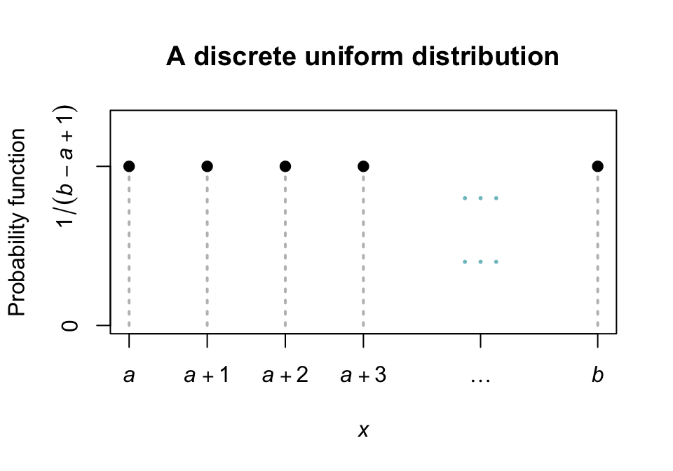
$The pf for the discrete uniform distribution $\text{Unif}(a, b)$$

Figure 4.1: The pf for the discrete uniform distribution $\text{Unif}(a, b)$

Definition 4.2 (Discrete uniform distribution: distribution function) For a random variable $X$ with the uniform distribution given by the probability function in (4.1), the distribution function is
\[ F_X(x; a, b) = \begin{cases} 0 & \text{for $x < a$}\\ \displaystyle \frac{\lfloor x\rfloor - a + 1}{b - a + 1} & \text{for $x = a, a + 1, \dots, b$}\\ 1 & \text{for $x > b$} \end{cases} \] where $\lfloor z \rfloor$ is the floor function (i.e., round $z$ to the nearest integer in the direction of $-\infty$).

Example 4.1 (Discrete uniform) Let $X$ be the number showing after a single throw of a fair die. Then $X \sim \text{Unif}(1, 6)$.

For an experiment involving selection of a single-digit number from a table of random digits, the number chosen, $X$, has probability distribution $\text{Unif}(0, 9)$.

The following are the basic properties of the discrete uniform distribution.

Theorem 4.1 (Discrete uniform properties) If $X\sim \text{Unif}(a, b)$ then

$\displaystyle \text{E}(X) = (a + b)/2$.
$\displaystyle \text{var}(X) = \frac{(b - a)(b - a + 2)}{12}$.
$\displaystyle M_X(t) = \frac {e^{at} - e^{(b + 1)t}}{(b - a + 1)(1 - e^{t})}$.

Proof. The mean and variance are easier to find by working with $Y = X - a$ rather than $X$ itself (as $Y$ is defined on $0 < y < (b - a)$), using that $\text{E}(X) = \text{E}(Y) + a$ and $\text{var}(Y) = \text{var}(X)$. Since $Y\sim\text{Unif}(0, b - a)$:
\[\begin{align*} \text{E}(Y) &= \sum_{y = 0}^{b - a} i\frac{1}{b - a + 1}\\ &= \frac{1}{b - a + 1}\big(0 + 1 + 2 + \dots + (b - a)\big)\\ &= \frac{(b - a)(b - a + 1)}{2(b - a + 1)} = (b - a)/2 \end{align*}\] using (A.1). Therefore,
\[ \text{E}(X) = \text{E}(Y) + a = \frac{b - a}{2} + a = \frac{a + b}{2}. \] The variance of $Y$ can be found similarly (Exercise 4.20).

To find the mgf:
\[\begin{align*} M_X(t) &= \sum_{x = a}^{b} \exp(xt) \frac{1}{b - a + 1}\\ &= \frac{1}{b - a + 1} \sum_{x = a}^{b} \exp(xt)\\ &= \frac{1}{b - a + 1} \left( \exp\{at\} + \exp\{(a + 1)t\} + \exp\{(a + 2)t\} + \dots + \exp\{bt\} \right) \\ &= \frac{\exp(at)}{b - a + 1} \left( 1 + \exp\{t\} + \exp\{2t\} + \dots + \exp\{(b - 1)t\} \right) \\ &= \frac{\exp(at)}{b - a + 1} \left( \frac{1 - \exp\{(b - a + 1)t\}}{1 - \exp(t)} \right) \end{align*}\] using (A.3).

4.3 Bernoulli distribution

A Bernoulli distribution is used in a situation where a single trial of a random process has two possible outcomes. A simple example is tossing a coin and observing if a head falls.

The probability function is simple:
\[ p_X(x) = \begin{cases} 1 - p & \text{if $x = 0$};\\ p & \text{if $x = 1$}, \end{cases} \] so that $p$ represents the probability of $x = 1$, called a ‘success’ (while $x = 0$ is called a ‘failure’). More succinctly:
\[\begin{equation} p_X(x; p) = p^x (1 - p)^{1 - x} \quad\text{for $x = 0, 1$}. \tag{4.2} \end{equation}\]

Definition 4.3 (Bernoulli distribution) Let $X$ be the number of successes in a single trial with $\Pr(\text{Success}) = p$ ($0\le p\le 1$). Then $X$ has a Bernoulli probability distribution with parameter $p$ and pf given by (4.2). We write $X\sim\text{Bern}(p)$.

Definition 4.4 (Bernoulli distribution: distribution function) For a random variable $X$ with the Bernoulli distribution given in (4.2), the distribution function is
\[ F_X(x; p) = \begin{cases} 0 & \text{if $x < 0$}\\ 1 - p & \text{if $0\leq x < 1$}\\ 1 & \text{if $x\geq 1$}. \end{cases} \]

The terms ‘success’ and ‘failure’ are not literal. ‘Success’ simply refers to the event of interest. If the event of interest is whether a cyclone causes damage, this is still called a ‘success’.

These ideas also introduces a common idea of a Bernoulli trial.

Definition 4.5 (Bernoulli trials) A Bernoulli trial is a random process with only two possible outcomes, usually labelled ‘success’ $s$ and ‘failure’ $f$. The sample space can be denoted by $S = \{ s, f\}$.

The following are the basic properties of the Bernoulli distribution.

Theorem 4.2 (Bernoulli distribution properties) If $X\sim\text{Bern}(p)$ then

$\text{E}(X) = p$.
$\text{var}(X) = p(1 - p) = pq$ where $q = 1 - p$.
$M_X(t) = pe^t + q$.

Proof. By definition:
\[ \text{E}(X) = \sum^1_{x = 0} x p_X(x) = 0\times (1 - p) + 1\times p = p. \] To find the variance, use the computational formula $\text{var}(X) = \text{E}(X^2) - \text{E}(X)^2$. Then,
\[ \text{E}(X^2) = \sum^1_{x = 0} x^2 p_X(x) = 0^2\times (1 - p) + 1^2\times p = p, \] and so
\[ \text{var}(X) = \text{E}(X^2) - \text{E}(X)^2 = p - p^2 = p (1- p). \]

The mgf of $X$ is
\[\begin{align*} M_X(t) &= \text{E}\big(\exp(tX)\big)\\ &= \sum^1_{x = 0} e^{tx} p^x q^{1 - x}\\ &= \sum^1_{x = 0}(pe^t)^x q^{1 - x} = pe^t + q. \end{align*}\] Proving the third result first, and then using it to prove the others, is easier (using of the methods in Sect. 3.6.2—try this as an exercise.)

4.4 Binomial distribution

A binomial distribution is used to model the number of successes in $n$ independent Bernoulli trials (Def. 4.5). A simple example is tossing a coin ten times and observing how often a head falls. The same random process is repeated (tossing the coin), only two outcomes are possible on each trial (a head or a tail), and the probability of a head remains constant on each trial (i.e., the tosses are independent).

4.4.1 Derivation of a binomial distribution

Consider tossing a die five times and observing the number of times a is rolled. The probability of observing a three times can be found as follows: In the five tosses, a must appear three times; there are $\binom{5}{3}$ ways of allocating on which of the five rolls they will appear. In the five rolls, must appear three times with probability $1/6$; the other two rolls must produce another number, with probability $5/6$. So the probability is
\[ \Pr(\text{3 ones}) = \binom{5}{3} (1/6)^3 (5/6)^2 = 0.032, \] assuming independence of the events. Using this approach, the pmf for the binomial distribution can be developed.

A binomial situation arises if a sequence of Bernoulli trials is observed, in each of which $\Pr(\{ s\} ) = p$ and $\Pr(\{ f\} ) = q = 1 - p$. For $n$ such trials, consider the random variable $X$, where $X$ is the number of successes in $n$ trials. Now $X$ will have value set $R_X = \{ 0, 1, 2, \dots, n\}$. $p$ must be constant from trial to trial, and the $n$ trials must be independent.

Consider the event $X = r$ (where $0\leq r\leq n$). This could correspond to the sample point
\[ \underbrace{s \quad s \quad s \dots s \quad s \quad s \quad s}_r\quad \underbrace{f \quad f \dots f \quad f}_{n - r} \] which is the intersection of $n$ independent events comprising $r$ successes and $n - r$ failures, and hence the probability is $p^r q^{n - r}$.

Every other sample point in the event $X = r$ will appear as a rearrangement of these $s$’s and $f$’s in the sample point described above and will therefore have the same probability.

Now the number of distinct arrangements of the $r$ successes $s$ and $(n - r)$ failures $f$ is $\binom{n}{r}$, so
\[ \Pr(X = r) = \binom{n}{r} p^r q^{n - r} \] for $r = 0, 1, \dots, n$. This is the binomial distribution.

Note that the sum of the probabilities is 1, as the binomial expansion of $(p + q)^n$ (using (A.4)) is
\[\begin{equation} \sum_{r = 0}^n \binom{n}{r} p^r q^{n - r} = (p + q)^n = 1\label{EQN:sumbin} \end{equation}\] since $p + q = 1$.

4.4.2 Definition and properties

The definition of the binomial distribution can now be given.

Definition 4.6 (Binomial distribution) Let $X$ be the number of successes in $n$ independent Bernoulli trials with $\Pr(\text{Success}) = p$ (for $0\le p\le 1$) constant for each trial. Then $X$ has a binomial probability distribution with parameters $n$, $p$ and pf given by
\[\begin{equation} p_X(x; n, p) = \binom{n}{x} p^x q^{n - x} \quad\text{for $x = 0, 1, \dots, n$}. \tag{4.3} \end{equation}\] We write $X\sim\text{Bin}(n, p)$.

The distribution function is complicated and is not given. Fig. 4.2 shows the pf for the binomial distribution for various parameter values.

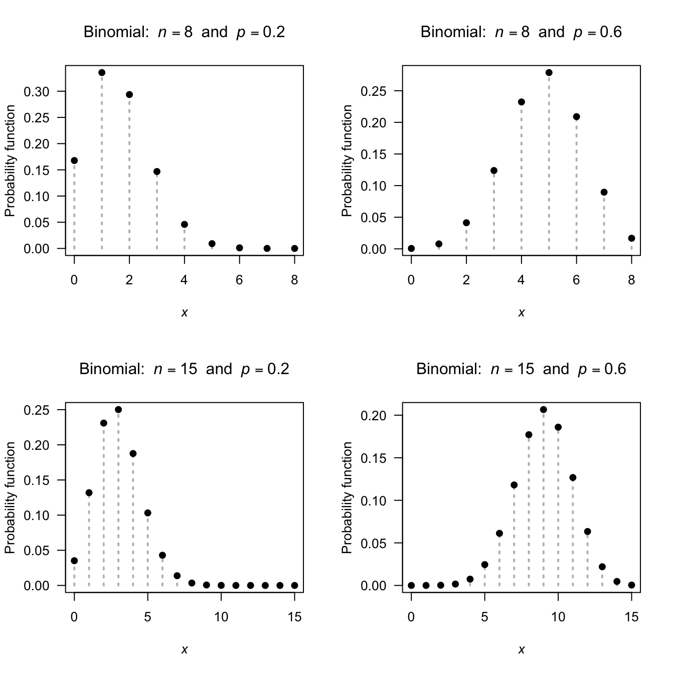
Figure 4.2: The pf for the binomial distribution for various values of $p$ and $n$

The following are the basic properties of the binomial distribution.

Theorem 4.3 (Binomial distribution properties) If $X\sim\text{Bin}(n,p)$ then

$\text{E}(X) = np$.
$\text{var}(X) = np(1 - p) = npq$.
$M_X(t) = (pe^t + q)^n$.

Proof. Using (A.4):
\[\begin{align*} \text{E}(X) & = \sum^n_{x = 0} x\binom{n}{x} p^x q^{n - x}\\ & = \sum^n_{x = 1} x \frac{n}{x} \binom{n - 1}{x - 1} p^x q^{n - x} \quad\text{(note the lower summation-index change)}\\ & = np\sum^n_{x = 1} \binom{n - 1}{x - 1} p^{x - 1} q^{n - x}\\ & = np \sum^{n - 1}_{y = 0} \binom{n - 1}{y}p^y q^{n - 1 - y}\quad \text{putting $y = x - 1$}. \end{align*}\] The summation is 1, since it is equivalent to summing over all values of $y$ for the binomial pf with $y$ successes in $(n - 1)$ Bernoulli trials, and hence represents a probability function with a sum of one. In the second line, the sum is over $x$ from $1$ to $n$ because, for $x = 0$, the probability is multiplied by $x = 0$ and makes no contribution to the summation. Thus,
\[ \text{E}(X) = np. \]

To find the variance, use the computational formula $\text{var}(X) = \text{E}(X^2) - \text{E}(X)^2$. Firstly, to find $\text{E}(X^2)$, write $\text{E}(X^2)$ as $\text{E}[X(X - 1) + X]$ so that $\text{E}[X(X - 1)] + \text{E}(X)$; then:
\[\begin{align*} \text{E}(X^2) &= \sum^n_{x = 0} x(x - 1)\Pr(X = x) + np\\ &= np + \sum^n_{x = 2} x(x -1)\frac{n(n - 1)}{x(x - 1)} \binom{n - 2}{x - 2} p^x q^{n - x}\\ &= np + \sum^n_{x = 2} n(n - 1)\binom{n - 2}{x - 2} p^x q^{n - x}\\ &= np + n(n - 1)p^2 \sum^{n - 2}_{y = 0} \binom{n - 2}{y} p^yq^{n - 2 - y}, \end{align*}\] putting $y = x - 2$. For the same reason as before, the summation is 1, so
\[ \text{E}(X^2) = np + n^2 p^2 - np^2 \] and hence
\[ \text{var}(X) = \text{E}(X^2) - [\text{E}(X)]^2 = np + n^2p^2 - np^2 - n^2 p^2 = np (1 - p). \]

The mgf of $X$ is
\[\begin{align*} M_X(t) &= \text{E}\big(\exp(tX)\big)\\ &= \sum^n_{x = 0} e^{tx}\binom{n}{x} p^x q^{n - x}\\ &= \sum^n_{x = 0}\binom{n}{x} (pe^t)^x q^{n - x} = (pe^t + q)^n. \end{align*}\] Proving the third result first, and then using it to prove the others, is easier (using of the methods in Sect. 3.6.2—try this as an exercise.)

Tables of binomial probabilities are commonly available, but computers (e.g., using R) can also be used to generate the probabilities. If the number of ‘successes’ has a binomial distribution, so does the number of ‘failures’. Specifically if $X\sim \text{Bin}(n,p)$, then $Y = (n - X) \sim \text{Bin}(n, 1 - p)$.

In R, many functions are built-in for computing the pf, df and other quantities for common distributions (see Appendix B).

The four R functions for working with the binomial distribution have the form [dpqr]binom(..., size, prob), where prob${} = p$ and size${} = n$. For example:

The function dbinom(x, size, prob) computes the probability function for the binomial distribution at $X = {}$x;
The function pbinom(q, size, prob) computes the distribution function for the binomial distribution at $X = {}$q;
The function qbinom(p, size, prob) computes the quantiles of the binomial distribution function for cumulative probability p; and
The function rbinom(n, size, prob) generates n random numbers from the given binomial distribution.

Example 4.2 (Throwing dice) A die is thrown 4 times. To find the probability of rolling exactly 2 sixes, see that there are $n = 4$ Bernoulli trials with $p = 1/6$. Let the random variable $X$ be the number of 6’s in 4 tosses. Then
\[ \Pr(X = 2) = \binom{4}{2} \left(\frac{1}{6}\right)^2\left(\frac{5}{6}\right)^2 = 150/1296 \approx 0.1157. \] In R:

dbinom(2,
       prob = 1/6,
       size = 4)
#> [1] 0.1157407

A binomial situation requires the trials to be independent, and the probability of success $p$ to be constant throughout the trials.

For example, drawing cards from a pack without replacing them is not a binomial situation; after drawing one card, the probabilities will then change for the drawing of the next card. In this case, the hypergeometric distribution should be used (Sect. 4.8).

Example 4.3 (Freezing lake) Based on Daniel S. Wilks (1995a) (p. 68), the probability that Cayuga Lake freezes can be modelled by a binomial distribution with $p = 0.05$.

Using this information, the number of times the lake will not freeze in $n = 10$ randomly chosen years in given by the random variable $X$ where $X \sim \text{Bin}(10, 0.95)$. The probability that the lake will not freeze in any of these ten years is $\Pr(X = 10) = \binom{10}{10} 0.95^{10} 0.05^{0} \approx 0.599$, or about 60%.

In R:

dbinom(0,
       size = 10,
       prob = 0.05)
#> [1] 0.5987369

Note we could define the random variable $Y$ as the number of times the lake will freeze in the ten randomly chosen years. Then, $Y\sim\text{Bin}(10, 0.05)$ and we would compute $\Pr(Y = 0)$ and get the same answer.

dbinom(10,
       size = 10,
       prob = 0.95)
#> [1] 0.5987369

Binomial probabilities can sometimes be approximated using the normal distribution (Sect. 5.3.4) or the Poisson distribution (Sect. 4.7.3).

4.5 Geometric distribution

4.5.1 Derivation of a geometric distribution

Consider now a random process where independent Bernoulli trials (Def. 4.5) are repeated until the first success occurs. What is the distribution of the number of failures until the first success is observed?

Let the random variable $X$ be the number of failures before the first success is observed. Since the first success may occur on the first trial, or second trial or third trial, and so on, $X$ is a random variable with range space $\{0, 1, 2, 3, \dots\}$ with no (theoretical) upper limit.

Since the probability of failure is $q = 1 - p$ and the probability of success is $p$, the probability of $x$ failures before the first success is
\[\begin{align*} \Pr(\text{$x$ failures}) &\times \Pr(\text{first success}) \\ q^x &\times p. \end{align*}\] This derivation assumes the events are independent.

4.5.2 Definition and properties

The definition of the geometric distribution can now be given.

Definition 4.7 (Geometric distribution) A random variable $X$ has a geometric distribution if the pf of $X$ is
\[\begin{equation} p_X(x; p) = (1 - p)^x p = q^x p\quad\text{for $x = 0, 1, 2, \dots$} \tag{4.4} \end{equation}\] where $q = 1 - p$ and $0 < p < 1$ is the parameter of the distribution. We write $X\sim\text{Geom}(p)$.

Definition 4.8 (Geometric distribution: distribution function) For a random variable $X$ with the geometric distribution given in (4.4), the distribution function is
\[ F_X(x; p) = \begin{cases} 0 & \text{for $x < 0$}\\ 1 - (1 - p)^{\lfloor x\rfloor + 1} & \text{for $x\ge 0$}, \end{cases} \] where $\lfloor z \rfloor$ is the floor function.

This is the parameterisation used by R. The pf for a geometric distribution for various values of $p$ is shown in Fig. 4.3. The following are the basic properties of the geometric distribution.

Theorem 4.4 (Geometric distribution properties) If $X\sim\text{Geom}(p)$ as defined in Eq. (4.4), then

$\text{E}(X) = (1 - p)/p$.
$\text{var}(X) = (1 - p)/p^2$.
$M_X(t) = p/\{1 - (1 - p)e^t\}$ for $t < -\log(1 - p)$.

Proof. The first two result can be proven directly but proving the third result, and using the mgf to prove the first two, is easier. This is left as an exercise (Ex. 4.21).

The four R functions for working with the geometric distribution have the form [dpqr]geom(prob), where prob${} = p$ (see Appendix B).

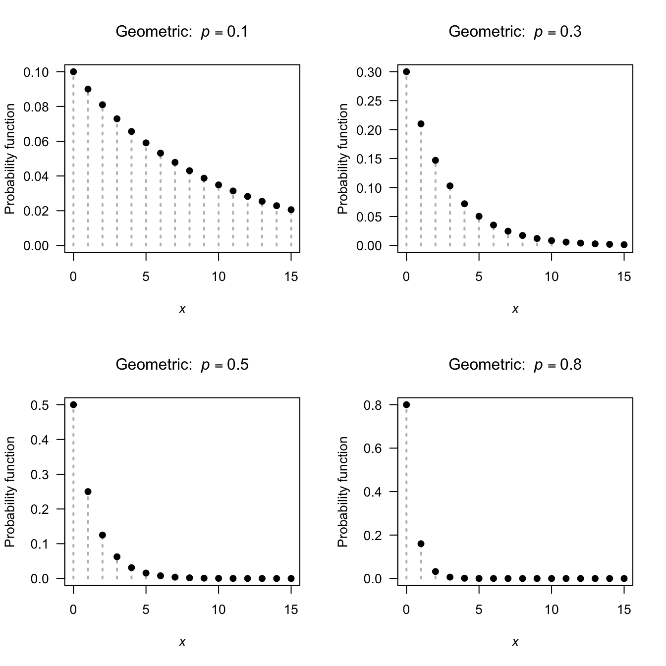
Figure 4.3: The pf for the geometric distribution for $p = 0.1$, $0.3$, $0.5$ and $0.8$

Example 4.4 (Netball shooting) Suppose a netball goal shooter has a probability of $p = 0.2$ of missing a goal. In this case a ‘success’ refers to missing the shot with $p = 0.2$

Let $X$ be the number of shots made till the first miss. Then, $X = \{1, 2, 3, \dots \}$, since the first miss may occur on the first shot, or any subsequent shot. This is not the parameterisation used by R.

Instead, let $Y$ be the number of goals scored until the shooter first misses. Notice that $Y = \{0, 1, 2, \dots \}$ so this parameterisation does correspond to that used by R, and $Y\sim \text{Geom}(0.2)$.

The probability that the shooter makes 4 goals before the first miss is:

dgeom(4, prob = 0.2)
#> [1] 0.08192

The probability that the shooter makes 4 or fewer goals before the first miss is $\Pr(Y = 0, 1, 2, 3, \text{or } 4)$:

pgeom(4, prob = 0.2)
#> [1] 0.67232

The expected number of shots until the first miss is $\text{E}(Y) = (1 - p)/p = 4$.

The parameterisation above is for the number of failures needed for the first success, so that $x = 0, 1, 2, 3, \dots$. An alternative parameterisation is for the number of trials $X$ before observing a success, when $x = 1, 2, \dots$. The only way to distinguish which parameterisation is being used is to check the range space or the pf.

Definition 4.9 (Geometric distribution: Alternative parameterisation) A random variable $X$ has a geometric distribution if the pf of $X$ is
\[\begin{equation} p_X(x) = (1 - p)^{x - 1}p = q^{x - 1} p\quad\text{for $x = 1, 2, \dots$} \tag{4.5} \end{equation}\] where $q = 1 - p$ and $0 < p < 1$ is the parameter of the distribution. We write $X\sim\text{Geom}(p)$.

Theorem 4.5 (Geometric distribution properties) If $X\sim\text{Geom}(p)$ as defined in Eq. (4.5), then

$\text{E}(X) = 1/p$.
$\text{var}(X) = (1 - p)/p^2$.
$M_X(t) = p\exp(t) /\{ 1 - (1 - p)e^t \}$ for $t < -\log(1 - p)$.

Proof. The first two result can be proven from Theorem 4.4.

4.6 Negative binomial distribution

4.6.1 Derivation: standard parameterisation

Consider a random process where independent Bernoulli trials are repeated until the $r$th success occurs. Let the random variable $X$ be the number of failures before the $r$th success is observed, so that $X = 0, 1, 2, \dots$.

To observe the $r$th success after $x$ failures, $x$ failures and $r - 1$ successes are observed first in these $x + r - 1$ trials. There are $\binom{x + r - 1}{r - 1}$ ways in which to allocate these successes to the first $x + r - 1$ trials. Each of the $r - 1$ successes occur with probability $p$, and the $x$ failures with probability $1 - p$ (assuming events are independent). Hence the probability of observing the $r$th success in trial $x$ is
\[\begin{align*} \text{No. ways} &\times \Pr\big(\text{$x$ failures}\big) \times \Pr(\text{$r - 1$ successes}) \\ \binom{x + r - 1}{r - 1} &\times (1 - p)^{x} \times p^{r - 1}. \end{align*}\]

4.6.2 Definition and properties: standard parameterisation

The standard definition of the negative binomial distribution can now be given.

Definition 4.10 (Negative binomial distribution) A random variable $X$ with pf
\[\begin{equation} p_X(x; p, r) = \binom{x + r - 1}{r - 1}(1 - p)^{x} p^{r - 1} \quad\text{for $x = 0, 1, 2, \dots$} \tag{4.6} \end{equation}\] has a negative binomial distribution with parameters $r$ (an positive integer) and $p$ ($0\le p\le 1$). We write $X\sim\text{NB}(r, p)$.

The distribution function is complicated and is not given. The following are the basic properties of the negative binomial distribution.

Theorem 4.6 (Negative binomial properties) If $X\sim \text{NB}(r, p)$ with pf (4.6) then

$\text{E}(X) = \{r(1 - p)\}/p$.
$\text{var}(X) = r(1 - p)/p^2$.
$M_X(t) = \left[ p / \{1 - (1 - p)\exp(t)\} \right]^r$ for $t < -\log p$.

Proof. Proving the third statement is left as an exercise. Then the first two are then derived from the mgf.

Example 4.5 (Negative binomial) A telephone marketer invites customers, over the phone, to a product demonstration. Ten people are needed for the demonstration. The probability that a randomly-chosen person accepts the invitation is only 0.15.

Here, a ‘success’ is an acceptance to attend the demonstration. Let $Y$ be the number of failed calls necessary to secure ten acceptances. Then $Y$ has a negative binomial distribution with $p = 0.15$ and $r = 10$. The mean number of failures made will is $\text{E}(Y) = \{r(1 - p)\}/p = \{10 \times (1 - 0.15)\}/0.15 \approx 56.66667$.

Hence, including the ten calls that leads to a person accepting the invitation, the mean number of calls to be made will is $10 + \text{E}(Y) = 66.66\dots$.

Since the parameterisation in (4.6) is defined over the non-negative integers, it is often used to model count data.

The four R functions for working with the negative binomial distribution are based on the paramaterisation in (4.6), and have the form [dpqr]nbinom(size, prob), where prob is $p$ and size is $r$ (see Appendix B).

The pf for the negative binomial distribution for various values of $p$ and $r$ is shown in Fig. 4.4.

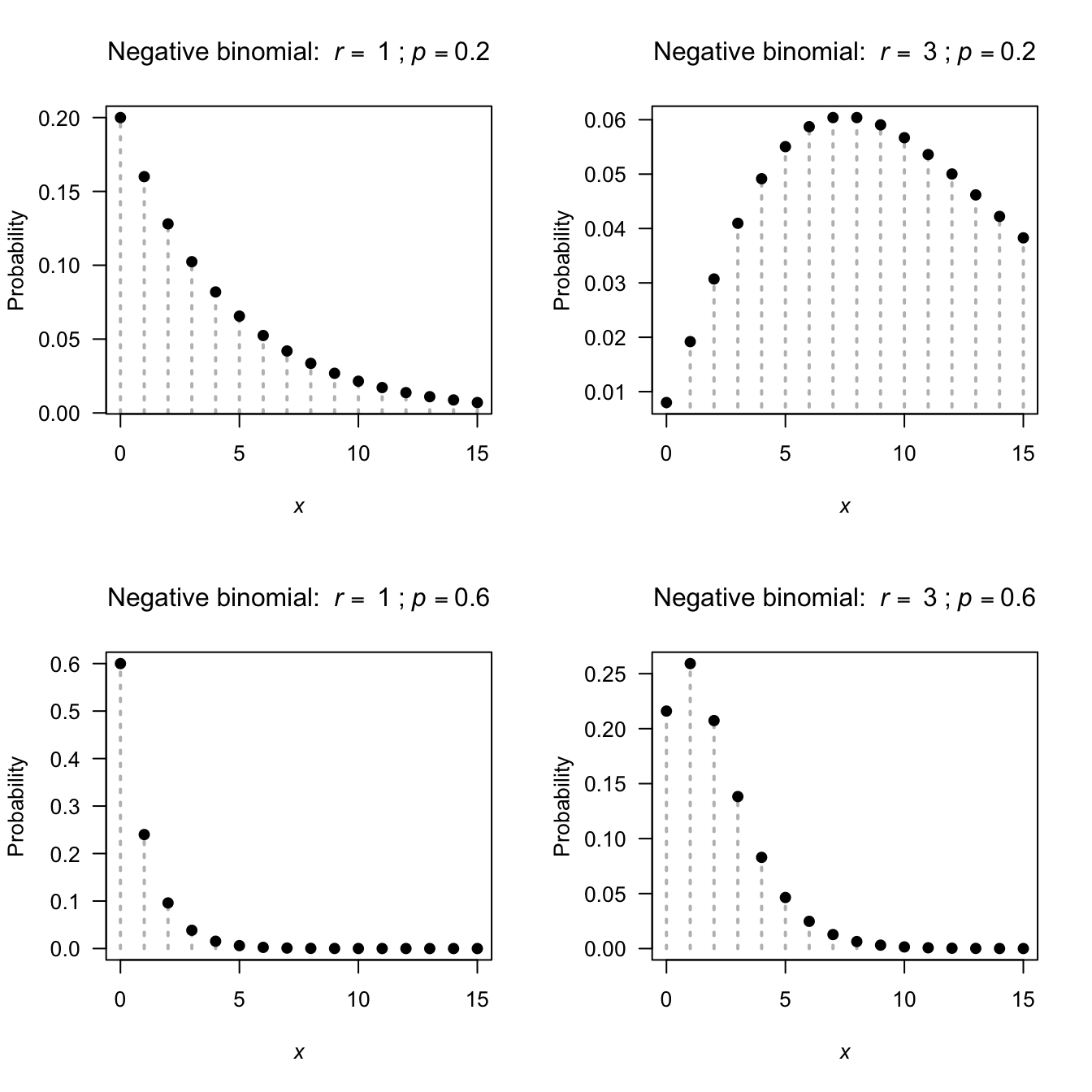
Figure 4.4: The pf for the negative binomial distribution for $p = 0.2$ and $0.7$ and $r = 1$ and $r = 3$

Example 4.6 (Negative binomial) Consider Example 4.5, concerning a telephone marketer inviting customers, over the phone, to a product demonstration. Ten people are needed for the demonstration. The probability that a randomly chosen person accepts the invitation is only $0.15$.

Consider finding the probability that the marketer will need to make more than $100$ calls to secure ten acceptances. In this situation, a ‘success’ is an acceptance to attend the demonstration. Let $Y$ be the number of failed calls before securing ten acceptances. Then $Y$ has a negative binomial distribution such that $Y\sim\text{NBin}(p = 0.15, r = 10)$.

To determine $\Pr(Y > 100) = 1 - \Pr(Y\le 100)$, using a computer is the easiest approach. In R, the command dnbinom() returns probabilities from the probability function of the negative binomial distribution, and pnbinom() returns the cumulative distribution probabilities:

x.values <- seq(1, 100, 
                by = 1)
1 - sum(dnbinom( x.values, 
                 size = 10, 
                 prob = 0.15))
#> [1] 0.02442528
# Alternatively:
1 - pnbinom(100, 
            size = 10, 
            prob = 0.15)
#> [1] 0.02442528

The probability is about $0.0244$.

Assuming each call take an average of 5 minutes, we can determine how long is the marketer expected to be calling to find ten acceptances. Let $T$ be the time to make the calls in minutes. Then $T = 5Y$. Hence, $\text{E}(T) = 5\text{E}(Y) = 5 \times 66.7 = 333.5$, or about 5.56 hours.

Assume that each call costs $25$ cents, and that the company pays the marketer $30 per hour. To determine the total cost, let $C$ be the total cost in dollars. The cost of employing the marketer is, on average, $30\times 5.56 = \$166.75$. Then $C = 0.25 Y + 166.75$, so $\text{E}(C) = 0.25 \text{E}(Y) + 166.75 = C = 0.25 \times 66.7 + 166.75 = \$183.43$.

4.6.3 Alternative parameterisations

Often, a different parameterisation for the negative binomial distribution; see Exercise 4.14. However, the parameterisation presented in Sect. 4.6.1 is used by R.

The negative binomial distribution can be extended so that $r$ can be any positive number, not just an integer. When $r$ is non-integer, the above interpretations are lost, but the distribution is more flexible. Relaxing the restriction on $r$ gives the pf as
\[\begin{equation} p_X(x; p, r) = \frac{\Gamma(x + r)}{\Gamma(r)\, x!} p^r (1 - p)^x, \tag{4.7} \end{equation}\] for $x = 0, 1, 2 \dots$ and $r > 0$. In this expression, $\Gamma(r)$ is the gamma function (Def. 4.11), and is related to factorials when $r$ is integer: $\Gamma(r) = (r - 1)!$ if $r$ is a positive integer.

Definition 4.11 (Gamma function) The function $\Gamma(\cdot)$ is called the gamma function and is defined as
\[ \Gamma(r) = \int_0^\infty x^{r - 1}\exp(-x)\, dx \] for $r > 0$.

The gamma function has the property that
\[\begin{equation} \Gamma(r) = (r - 1)! \tag{4.8} \end{equation}\] if $r$ is a positive integer (Fig. 4.5). Important properties of the gamma function are given below.

Theorem 4.7 (Gamma function properties) For the gamma function $\Gamma(\cdot)$,

$\Gamma(r) = (r - 1)\Gamma(r - 1)$ if $r > 0$.
$\Gamma(1/2) = \sqrt{\pi}$.
$\lim_{r\to 0} \to \infty$.
$\Gamma(1) = \Gamma(2) = 1$.
$\Gamma(n) = (n - 1)$ for all positive integers $n$.

Proof. For the first property, integration by parts gives
\[\begin{align*} \Gamma(r) &= \left. -\exp(-x) \frac{x^2}{r}\right|_0^\infty + \int_0^\infty \exp(-x) (r - 1) x^{r - 2}\,dx\\ &= 0 + \ (r - 1) \int_0^{\infty} e^{-x} x^{r - 2} \, dx\\ &= (r - 1) \Gamma(r - 1). \end{align*}\]

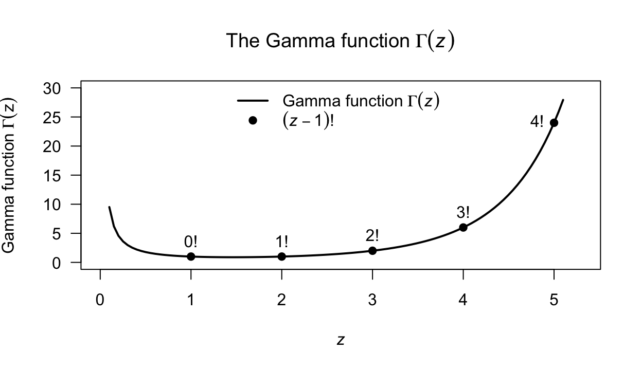
$The gamma function is like the factorial function but has a continuous argument. The line corresponds to the gamma function $\Gamma(z)$; the solid points correspond to the factorial $(z - 1)! = \Gamma(z)$ for integer $z$.$

Figure 4.5: The gamma function is like the factorial function but has a continuous argument. The line corresponds to the gamma function $\Gamma(z)$; the solid points correspond to the factorial $(z - 1)! = \Gamma(z)$ for integer $z$.

Example 4.7 (Negative binomial) Consider a computer system that fails with probability $p = 0.02$ on any given day (so that the system failure is a ‘success’). Suppose after five failures, the system is upgraded.

To find the probability that an upgrade will happen within one year, let $D$ be the number of days before the fifth failure. So, we seek $\Pr(X < 360)$. Using R:

pnbinom(360, 
        size = 5, 
        prob = 0.02)
#> [1] 0.8553145

So the probability of upgrading within one year is about $85$%.

Example 4.8 (Mites) Bliss (1953) gives data from the counts of adult European red mites on leaves selected at random from six similar apple trees (Table 4.1). The mean number of mites per leaf is 1.14 witha variance of 3.57; The Poisson distribution has an equal mean and variance, the Poisson distribution may not model these count data well. However, the mean number of mites per leaf can be modelled using a negative binomial distribution with $r = 1.18$ and $p = 0.5$.

the estimated probability function for both the Poisson and negative binomial distributions are given in Table 4.1; the negative binomial distribution fits better as expected.

Table 4.1: Counts of mites on leaves selected at random from six similar apple trees
No. leaves	No. mites	Empirical prob.	Poisson prob.	Neg. bin. prob.
0	70	0.467	0.318	0.449
1	38	0.253	0.364	0.261
2	17	0.113	0.209	0.140
3	10	0.067	0.080	0.073
4	9	0.060	0.023	0.038
5	3	0.020	0.005	0.019
6	2	0.013	0.001	0.010
7	1	0.007	0.000	0.005
8+	0	0.000	0.000	0.000

4.7 Poisson distribution

The Poisson distribution is very commonly used to model the number of occurrences of an event which occurs randomly in time or space. The Poisson distribution arises as a result of assumptions made about a random process:

Events that occur in one time-interval (or region) are independent of those occurring in any other non-overlapping time-interval (or region).
The probability that an event occurs in a small time-interval is proportional to the length of the interval.
The probability that 2 or more events occur in a very small time-interval is so small that it is negligible.

Whenever these assumptions are valid, or approximately so, the Poisson distribution is appropriate. Many natural phenomena fall into this category.

4.7.1 Derivation of Poisson distribution

The binomial distribution applies in situations where an event may occur a certain number of times in a fixed number of trials, say $n$. What if $n$ gets increasingly large though, so effectively there is no upper limit? Mathematically, we might say: What happens if $n\to\infty$?

Let’s find out. Begin with the binomial probability function
\[\begin{equation} p_X(x; n, p) = \binom{n}{x} p^x (1 - p)^{n - x} \quad\text{for $x = 0, 1, \dots, n$} \tag{4.9} \end{equation}\] which has a mean of $\lambda = np$. First, re-writing (4.9) in terms of the mean $\lambda$:
\[\begin{equation} p_X(x; n, \lambda) = \binom{n}{x} \left(\frac{\lambda}{n}\right)^x \left(1 - \frac{\lambda}{n}\right)^{n - x} \quad\text{for $x = 0, 1, \dots, n$}. \tag{4.10} \end{equation}\] Now consider the case $n \to \infty$ (for $x = 0, 1, \dots$):
\[\begin{align} \lim_{n\to\infty} p_X(x; n, \lambda) &= \lim_{n\to\infty} \binom{n}{x} \left(\frac{\lambda}{n}\right)^x \left(1 - \frac{\lambda}{n}\right)^{n - x}\\ &= \frac{\lambda^x}{x!} \lim_{n\to\infty} \frac{n!}{(n - x)!} \frac{1}{n^x} \left(1 - \frac{\lambda}{n}\right)^{n} \left(1 - \frac{\lambda}{n}\right)^{-x}. \end{align}\] Now, since the limit of product of functions is equal to product of their limits, each component can be considered in turn.

Looking at the first component, see that
\[\begin{align} \lim_{n\to\infty} \frac{n!}{(n - x)!} \times \frac{1}{n^x} &= \lim_{n\to\infty} \frac{n \times (n - 1) \times (n - 2) \times\cdots\times 2 \times 1} {(n - x)\times (n - x - 1) \times \cdots \times 2 \times 1} \times \frac{1}{n^x}\\ &= \lim_{n\to\infty}\frac{ \overbrace{n \times (n - 1) \times \cdots\times (n - x + 1)}^{\text{$x$ terms}}} { \underbrace{n \times n \times\cdots \times n\times n}_{\text{$x$ terms}}}\\ &= \lim_{n\to\infty} \frac{n}{n} \times \frac{n - 1}{n} \times \frac{n - 2}{n} \times\cdots\times \frac{n - x + 1}{n}\\ &= 1 \times 1\times\cdots\times 1 = 1. \end{align}\] For the next component, see that (using (A.10)):
\[ \lim_{n\to\infty} \left(1 - \frac{\lambda}{n}\right)^{n} = \exp(-\lambda). \] For the last term:
\[ \lim_{n\to\infty} \left(1 - \frac{\lambda}{n}\right)^{-x} = 1^{-x} = 1. \] Putting the pieces together:
\[\begin{align} \lim_{n\to\infty} p_X(x; n, \lambda) &= \frac{\lambda^x}{x!} \lim_{n\to\infty} \frac{n!}{(n - x)!} \frac{1}{n^x} \left(1 - \frac{\lambda}{n}\right)^{n} \left(1 - \frac{\lambda}{n}\right)^{-x}\\ p_X(x; \lambda) &= \frac{\lambda^k}{x!} 1 \times \exp(-\lambda) \times 1\\ &= \frac{\exp(-\lambda) \lambda^x}{x!}, \end{align}\] for $x = 0, 1, 2, \dots$. This is the probability function for the Poisson distribution.

A Poisson process refers to events that occur at a rate $\lambda$, but occur at random.

4.7.2 Definition and properties

The definition of the Poisson distribution can now be given.

Definition 4.12 (Poisson distribution) A random variable $X$ is said to have a Poisson distribution if its pmf is
\[\begin{equation} p_X(x; \lambda) = \frac{\exp(-\lambda) \lambda^x}{x!}\quad \text{for $x = 0, 1, 2, \dots$} \tag{4.11} \end{equation}\] where the parameter is $\lambda > 0$. We write $X\sim\text{Pois}(\lambda)$.

Definition 4.13 (Poisson distribution: distribution function) For a random variable $X$ with the Poisson distribution given in (4.11), the distribution function is
\[ F_X(x; \lambda) = \begin{cases} 0 & \text{for $x < 0$}\\ \displaystyle \exp(-\lambda) \sum _{i = 0}^{\lfloor x \rfloor }{\frac {\lambda ^{i}}{i!}} & \text{for $x\ge 0$};\\ \end{cases} \] where $\lfloor z \rfloor$ is the floor function.

The pmf for a Poisson distribution for different values of $\lambda$ is shown in Fig. 4.6.

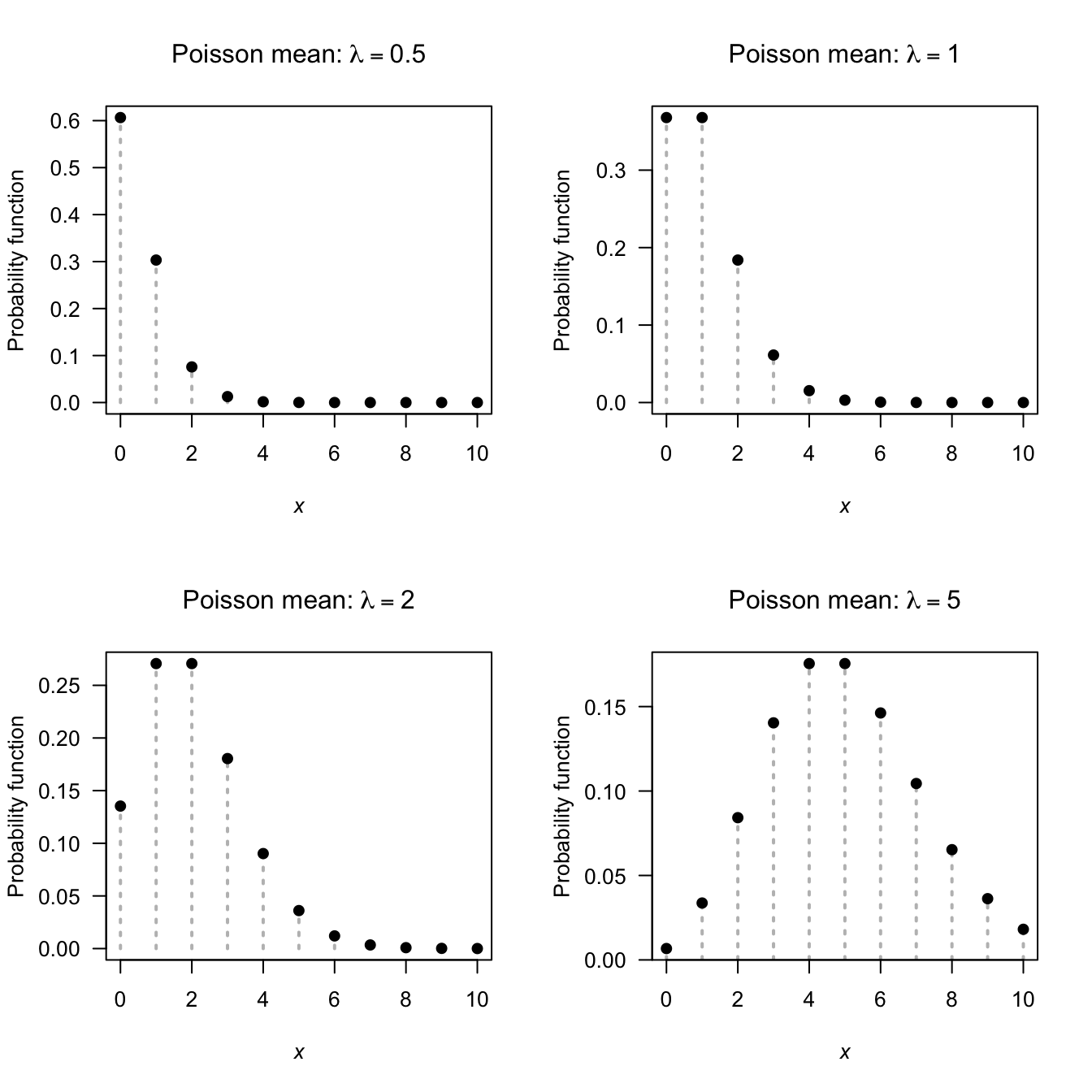
$The pf for the Poisson distribution for various values of $\lambda$$

Figure 4.6: The pf for the Poisson distribution for various values of $\lambda$

The following are the basic properties of the Poisson distribution.

Theorem 4.8 (Poission distribution properties) If $X\sim\text{Pois}(\lambda)$ then

$\text{E}(X) = \lambda$.
$\text{var}(X) = \lambda$.
$M_X(t) = \exp[ \lambda\{\exp(t) - 1\}]$.

Proof. The third result is proven, then the other results follow:
\[\begin{align*} M_X(t) = \text{E}(e^{tX}) &= \sum^\infty_{x = 0} e^{xt} e^{-\lambda} \lambda^x / x!\\ &= e^{-\lambda} \sum^\infty_{x = 0} \frac{(\lambda\, e^t)^x}{x!} \\ &= e^{-\lambda} \left[ 1 + \lambda\, e^t + \frac{(\lambda\,e^t)^2}{2!} + \dots \right]\\ &= e^{-\lambda} e^{\lambda\, e^t}\\ &= e^{-\lambda (1 - e^t)}, \end{align*}\] using (A.8). The first two results follow from differentiating the mgf.

Notice that the Poisson distribution has the variance equal to the mean. The negative binomial distribution has two parameters and the Poison only one, so often the negative binomial distribution produces a better fit to data.

The four R functions for working with the Poisson distribution have the form [dpqr]poiss(lambda) (see Appendix B).

Example 4.9 (Queuing) Customers enter a service line ‘at random’ at a rate of 4 per minute. Assume that the number entering the line in any given time interval has a Poisson distribution. To determine the probability that at least one customer enters the line in a given $\frac{1}{2}$-minute interval, use (since $\lambda = 2$ over half-hour):
\[ \Pr(X\geq 1) = 1 - \Pr(X = 0) = 1 - e^{-2} = 0.865. \] In R:

1 - dpois(0,
          lambda = 2)
#> [1] 0.8646647

Example 4.10 (Bomb hits) Clarke (1946) (quoted in Hand et al. (1996), Dataset 289) discusses the number of flying bomb hits on London during World War II in a 36 square kilometre area of South London. The area was gridded into 0.25 km squares and the number of bombs falling in each grid was counted (Table 4.2). Assuming random hits, the Poisson distribution can be used to model the data using $\lambda = 0.93$. The pf for the Poisson distribution can be compared to the empirical probabilities computed above; see Table 4.2. For example, the probability of zero hits is
\[ \frac{\exp(-0.93) (0.93)^0}{0!} \approx 0.39. \] The two probabilities are very close; the Poisson distribution fits the data very well.

Table 4.2: The number of flying bomb hits on London during World War II in a 36 square kilometre area of South London. The proportion of the 576 grid squares receiving 0, 1, …hits was also computed. The observed and empirical probabilities are shown. The Poisson distribution fits the data well.
Hits	Number bombs	Proportion bombs	Poisson proportion
0	229	0.3976	0.3946
1	211	0.3663	0.3669
2	93	0.1615	0.1706
3	35	0.0608	0.0529
4	7	0.0122	0.0123
5	0	0.0000	0.0023
6	0	0.0000	0.0004
7	1	0.0017	0.0000

4.7.3 Relationship to the binomial distribution

Given the derivation of the Poisson distribution (Sect. 4.7.1), a relationship between the Poisson and binomial distributions should come as no surprise.

Computing binomial probabilities is tedious if the number of trials $n$ is very large and the probability of success in a single trial is very small. For example, consider $X\sim \text{Bin}(n = 2000, p = 0.005)$; the pf is
\[ p_X(x) = \binom{2000}{x}(0.005)^x 0.995^{2000 - x}. \] Using the pmf, computing some probabilities, such as $\Pr(X > 101)$, is tedious. (Try computing $\binom{2000}{102}$ on your calculator, for example.) However, the Poisson distribution can be used to approximate this probability.

Set the Poisson mean to equal the binomial mean (that is, $\lambda = \mu = np$). Since $\text{E}(Y) = \text{var}(Y) = \lambda$ for the Poisson distribution, this means the variance is also set to $\sigma^2 = np$. Of course, the binomial mean is $np(1 - p)$, so this can only be (approximately) true if $p$ is close to zero (and so $1 - p\approx 1$).

A general guideline is that the Poisson distribution can be used to approximate the binomial when $n$ is large (recall, the derivation was for the case $n\to\infty$), $p$ is small and $np \le 7$.

The Poisson distribution is an excellent approximation to the binomial distribution when $p$ is small and $n$ is large. The binomial pf is shown using empty circles; the Poisson pf using crosses.

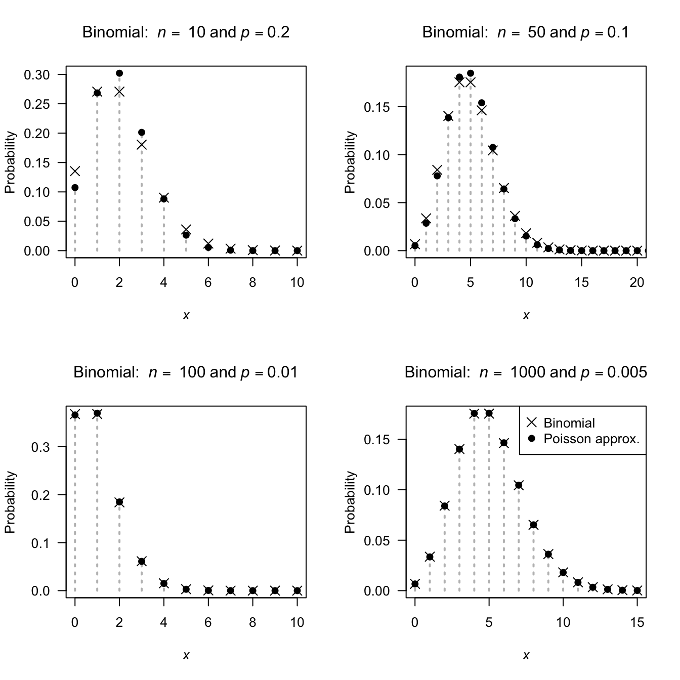
Figure 4.7: The Poisson distribution is an excellent approximation to the binomial distribution when $p$ is small and $n$ is large. The binomial pf is shown using empty circles; the Poisson pf using crosses.

4.7.4 Extensions

The Poisson distribution is commonly used to model independent counts. However, sometimes these counts explicitly exclude a count of zero. For example, consider modelling the number of nights patients spend in hospital; patients must spend at least one night to be in the data. Then, the probability functions can be expressed as
\[ p_X(x; \lambda) = \frac{\exp(-\lambda) \lambda^{x - 1}}{(x - 1)!}\quad \text{for $x = 1, 2, 3, \dots$} \] where the parameter is $\lambda > 0$. This is called the zero-truncated Poisson distribution. In this case, $\text{E}(X) = \lambda + 1$ and $\text{var}(X) = \lambda$ (Ex. 4.22).

In some cases, the random variable is a count, but has an upper limit on the possible number of counts. This is the truncated Poisson distribution.

Other situations exist where the the proportions of zeros exceed the proportions expected by the Poisson distribution (e.g., $\exp(-\lambda)$), but the Poisson distributions seems to otherwise be suitable. In these situations, the zero-inflated Poisson distribution may be suitable.

4.8 Hypergeometric distribution

4.8.1 Derivation of a hypergeometric distribution

When the selection of items a fixed number of times is done with replacement, the probability of an item being selected stays the same and the binomial distribution can be used. However, when the selection of items is done without replacement, the trials are not independent, making the binomial model unsuitable. In these situations, a hypergeometric distribution is appropriate.

Consider a simple example: A bag contains six light-coloured balls and four dark-coloured balls (Fig. 4.8). The variable of interest, say $X$, is the number of light-coloured balls drawn in three random selections from the bag, without replacing the balls. Since the balls are not replaced, $\Pr(\text{draw a light-coloured ball})$ is not constant, and so the binomial distribution cannot be used.

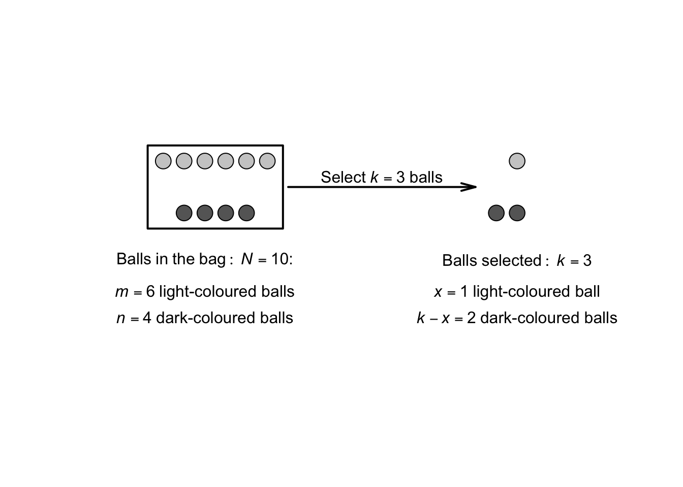
Figure 4.8: Drawing balls from a ‘bag’

The probabilities can be computed, however, using the counting ideas from Chap. 1. There are a total of $\binom{10}{3}$ ways of selecting a sample of size $k = 3$ from the bag. Consider the case $X = 0$. The number of ways of drawing no light-coloured balls is $\binom{6}{0}$ and the number of ways of drawing the three dark-coloured balls in $\binom{4}{3}$, so the probability is
\[ \Pr(X = 0) = \frac{\binom{6}{0}\binom{4}{3}}{\binom{10}{3}} \approx 0.00833. \] Likewise, the number of ways to draw one light-coloured ball (and hence two dark-coloured balls; Fig. 4.8) is $\binom{6}{1}\times \binom{4}{2}$, so
\[ \Pr(X = 1) = \frac{ \binom{6}{1}\times \binom{4}{2} }{\binom{10}{3}}. \] Similarly,
\[ \Pr(X = 2) =\frac{ \binom{6}{2}\times \binom{4}{1} }{\binom{10}{3}} \quad\text{and}\quad \Pr(X = 3) =\frac{ \binom{6}{3}\times \binom{4}{0} }{\binom{10}{3}}. \]

4.8.2 Definition and properties

In general, suppose a bag contains $N$ balls, and $m$ of them are light-coloured and $n$ and not light-coloured; then $N = m + n$. Suppose a sample of size $k$ is drawn from the bag without replacement; then the probability of finding $x$ light-coloured balls in the sample of size $k$ is
\[ \Pr(X = x) = \frac{ \binom{m}{x}{ \binom{n}{k - x}}}{\binom{N}{k}} = \frac{ \binom{m}{x}{ \binom{n}{k - x}}}{\binom{m + n}{k}} \] where $X$ is the number of light-coloured balls in sample of size $k$. (In the example, $k = 3$, $m = 6$ and $N = 10$.)

In the formula, $\binom{m}{x}$ is the number of ways of selecting $x$ light-coloured balls from the $m$ light-coloured balls in the bag; $\binom{n}{k - x}$ is the number of ways of selecting all the remaining $k - x$ to be the other colour (and there are $n = N - m$ of those in the bag); and $\binom{N}{k}$ is the number of ways of selecting a sample of size $k$ if there are $N$ balls in the bag in total.

Definition 4.14 (Hypergeometric distribution) Consider a set of $N = m + n$ items of which $m$ are of one kind (call them ‘successes’) and other $n = N - m$ are of another kind (call them ‘failures’). We are interested in the probability of $x$ successes in $k$ trials, when the selection (or drawing) is made without replacement. Then the random variable $X$ is said to have a hypergeometric distribution with pf
\[\begin{equation} p_X(x; n, m, k) = \frac{ \binom{m}{x}\binom{n}{k - x}}{\binom{m + n}{k}} \tag{4.12} \end{equation}\] where $\max(0, k - n) \le x \le \min(n, m)$.

The distribution function is complicated and is not given. The following are the basic properties of the hypergeometric distribution.

Theorem 4.9 (Hypergeometric distribution properties) If $X$ has a hypergeometric distribution with pf (4.12), then (writing $N = m + n$)

$\text{E}(X) = km/N$.
$\displaystyle \text{var}(X) = k \left(\frac{m}{N}\right)\left(\frac{N - k}{N - 1}\right)\left(1 - \frac{m}{N}\right)$.

The moment-generating function is difficult and will not be considered.

The four R functions for working with the hypergeometric distribution functions have the form [dpqr]hyper(m, n, k), where k${} = k$, m${} = m$ and m${} + {}$n${} = N$, so that n${}={}$N${}-{}$m (see Appendix B).

Consider the example at the start of this section. The probability of drawing a light-coloured ball initially is $6/10 = 0.6$, and the probability that the next ball is light-coloured is $5/9 = 0.556$. But suppose there are 10,000 balls in the bag, of which 6000 are light-coloured. The probability of drawing a light-coloured ball initially is $6000 / 10,000 = 0.6$, and the probability that the next ball is light-coloured becomes $5999/9999 = 0.59996$; the probability is almost the same. In this case, we might consider using the binomial distribution with $p\approx 0.6$.

In general, if $N$ is much larger than $k$, the population proportion then will be approximately $p\approx m/N$, and so $1 - p \approx (N - m)/N$. Using this information,
\[ \text{E}(X) = k \times (m/N) \approx kp \] and \[\begin{align*} \text{var}(X) &= k\left(\frac{m}{N}\right)\left(1 - \frac{m}{N}\right)\left(\frac{N - k}{N - 1}\right)\\ &\approx k\left( p \right ) \left( 1 - p \right) \left(1 \right ) \\ &= k p (1 - p), \end{align*}\] which correspond to the mean and variance of the binomial distribution.

Example 4.11 (Mice) Twenty mice are available to be used in an experiment; seven of the mice are female and $13$ are male. Five mice are required and will be sacrificed. What is the probability that more than three of the mice are males?

Let $X$ be the number of male mice chosen in a sample of size $k = 5$. Then $X$ has a hypergeometric distribution (since mice are chosen without replacement) where $N = 20$, $k = 5$, $m = 13$ and $n = 20 - 13 = 7$, and we seek
\[\begin{align*} \Pr(X > 3) &= \Pr(X = 4) + \Pr(X = 5) \\ &= \frac{ \binom{13}{4} \binom{7}{1}}{ \binom{20}{5} } + \frac{ \binom{13}{5} \binom{7}{0}}{ \binom{20}{5} } \\ & \approx 0.3228 + 0.0830 = 0.4058. \end{align*}\] The probability is about 41%:

dhyper(x = 4, m = 13, n = 7, k = 5) + 
  dhyper(x = 5, m = 13, n = 7, k = 5)
#> [1] 0.4058308

4.9 Simulation

Distributions can be used to simulate practical situations, using random numbers generated from the distributions. In R, these function start with the letter r; for example, to generate three random numbers from a Poisson distribution, use rpois():

rpois(3, # Generate three random numbers...
      lambda = 4) # ... with mean = 4
#> [1] 2 4 4

Consider a study of insects where a females lays $E$ eggs, only some of which are fertile (based on Ito (1977)). Suppose $E \sim \text{Pois}(8.5)$, and the probability that any given egg is fertile is $p = 0.6$ (and assume the fertility of the eggs from any one female are independent).

The fertility for one females can be modelled in R:

# One female
NumberOfEggs <- rpois(1, 
                      lambda = 8.5)

# How many eggs are fertile?
NumberFertileEggs <- rbinom(1, # Only one random number for this one female
                            size = NumberOfEggs,
                            prob = 0.6)
cat("Number of eggs:", NumberOfEggs,
    "| Number of fertile eggs:", NumberFertileEggs, "\n")
#> Number of eggs: 5 | Number of fertile eggs: 3

Since random numbers are being generated, each simulation will produce different results, so we repeat this over many simulations:

# Many simulations

numberSims <- 5000

NumberOfEggs <- array( dim = numberSims )
NumberFertileEggs <- array( dim = numberSims )

for (i in (1:numberSims)){ 
  NumberOfEggs[i] <- rpois(1, lambda = 8.5)
  
  # How many fertile?
  NumberFertileEggs[i] <- rbinom(1, # Only one random number/female
                                 size = NumberOfEggs[i],
                                 prob = 0.6)
}

We can then draw a histogram of the number of fertile eggs laid by females (Fig. 4.9):

hist(NumberFertileEggs,
     las = 1, # Horizontal tick mark labels
     xlab = "Number of fertile eggs",
     ylab = "Count",
     main = "Number of fertile eggs:\n5000 simulations")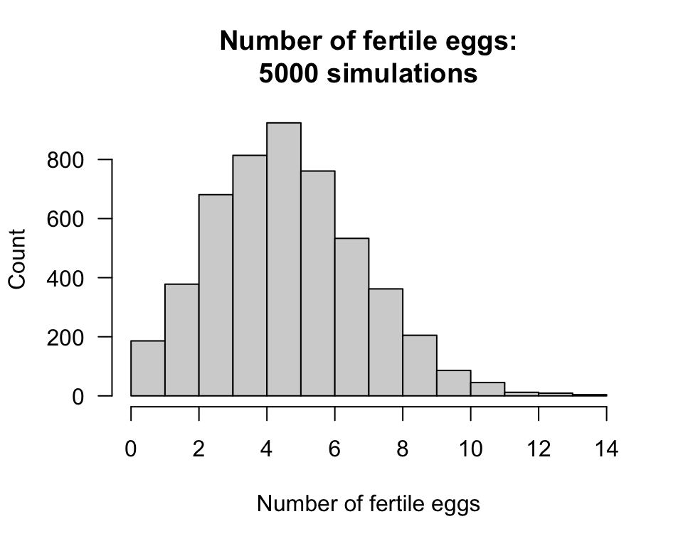

Figure 4.9: The number of fertile eggs laid, over 5000 simulations

Using this information, questions can be answered about the number of fertile eggs layed. For example:

sum( NumberFertileEggs > 6) / numberSims
#> [1] 0.2512

The chance that a female lays more than 6 fertile eggs is about 25.1%. The mean and variance of the number of fertile eggs laid is:

mean( NumberFertileEggs )
#> [1] 5.1074
var( NumberFertileEggs )
#> [1] 4.97166

4.10 Exercises

Exercise 4.1 If $X \sim \text{Bin}(n, 1 - p)$, show that $(n - X) \sim \text{Bin}(n, p)$.

Exercise 4.2 A study by Sutherland et al. (2012) found that about 30% of Britons ‘generally added salt’ at the dinner table.

In a group of 25 Britons, what is the probability that at least 10 added salt?
In a group of 25 Britons, what is the probability that no more than 9 added salt?
In a group of 25 Britons, what is the probability that between 5 and 10 (inclusive) added salt?
What is the probability that 6 Britons would need to be selected to find one that adds salt?
What is the probability that at least 8 Britons would need to be selected to find the first that add salt?
What is the probability that at least 8 Britons would need to be selected to find three that add salt?
What assumptions are being made in the above calculations?

Exercise 4.3 A study by Loyeung et al. (2018) examined whether people could identify potential placebos. The 81 subjects were each presented with five different supplements, and asked to select which one was the legitimate herbal supplement based on the taste (the rest were placebos).

What is the probability that more than 15 will correctly identify the legitimate supplement?
What is the probability that at least 12 correctly identify the legitimate supplement?
What is the probability that the first person to identify the legitimate supplement is the third person tested?
What is the probability that the fifth person to identify the legitimate supplement is the 10th person tested?
In the study, 50 people correctly selected the true herbal supplement. What does this suggest?

Exercise 4.4 A study by Maron (2007) used statistical modelling to show that the mean number of noisy miners (a type of bird) in sites with about 15 eucalypts per two hectares was about 3.

In a two hectare site with 15 eucalypts, what is the probability of observing no noisy miners?
In a two hectare site with 15 eucalypts, what is the probability of observing more than 5 noisy miners?
In a four hectare site with 30 eucalypts, what is the probability of observing two noisy miners?

Exercise 4.5 In a study of rainfall disaggregation (Connolly, Schirmer, and Dunn 1998) (extracting small-scale rainfall features from large-scale measurements), the number of non-overlapping rainfall events per day at Katherine was modelled using a Poisson distribution (for $x = 1, 2, 3, \dots$) with $\lambda = 2.5$ in summer and $\lambda = 1.9$ in winter.

Denote the number of rainfall events in summer as $S$, and in winter as $W$.

Plot the two distributions, and compare summer and winter (on the same graph). Compare and comment.
What is the probability of more than 3 rainfall events per day in winter?
What is the probability of more than 3 rainfall events per day in summer?
Describe what is meant by the statement $\Pr(S > 3 \mid S > 1)$, and compute the probability.
Describe what is meant by the statement $\Pr(W > 2 \mid W > 1)$, and compute the probability.

Exercise 4.6 Consider a population of animals of a certain species of unknown size $N$ (Romesburg and Marshall 1979). A certain number of animals in an area are trapped and tagged, then released. At a later point, more animals are trapped, and the number previously tagged is noted.

Define $p$ as the probability that an animal is captured zero times during the study, and $n_x$ as the number of animals captured $x$ times (for $x = 0, 1, 2, \dots$). ($n_0$, which we write as $N$, is unknown.) The study consist of $s$ trapping events, so we have $n_1$, $n_2, \dots n_s$ where $s$ is sufficiently ‘large’ that the truncation is negligible. Then,
\[\begin{equation} n_x = N p (1 - p)^x \quad \text{for $x = 0, 1, 2, \dots$}. \tag{4.13} \end{equation}\] While $p$ and $N$ are both unknown, the value of $N$ is of interest

Explain how (4.13) arises.
Take logarithms of both sides of of (4.13), and hence write this equation in the form of a linear regression equation $\hat{y} = \beta_0 + \beta_1 x$.
From the regression equation, identify how to estimate $p$ from the slope of the regression line ($\beta_1$), and then $N$ from the $y$-intercept ($\beta_0$).
Use the data in Table 4.3, from a study of rabbits in an area Michigan (Eberhardt, Peterle, and Schofield 1963), to estimate the rabbit population.

(Hint: To fit a regression line in R, use lm(); for example, to fit the regression line $\hat{y} = \beta_0 + \beta_1 x$, use lm(y ~ x).)

Table 4.3: The number of rabbits $n_x$ at each trapping who had been previously trapped
$x$	1	2	3	4	5	6
$n_x$	247	63	20	4	2	1

Exercise 4.7 A Nigerian study of using solar energy to disinfect water (SODIS) modelled the number of days exposure needed to disinfect the water (Nwankwo and Attama 2022). The threshold for disinfection was a single day recording 4 kWh/m² daily cumulative solar irradiance. Define $p$ as the probability that a single day records more than this threshold.

Suppose $p = 0.5$. How many days exposure would be needed, on average, to achieve disinfection?
Suppose $p = 0.25$. How many days exposure would be needed, on average, to achieve disinfection?
If $p = 0.25$, what is the variance of the number of days needed to achieve disinfection?
If $p = 0.25$, what is the probability that disinfection will be achieved in three days or fewer?

Exercise 4.8 A negative binomial distribution was used to model the number of parasites on feral cats on on Kerguelen Island (Hwang, Huggins, and Stoklosa 2016). The model used is parameterised so that $\mu = 8.7$ and $k = 0.4$, where $\text{var}(X) = \mu + \mu^2/k$.

Use the above information to determine the negative binomial parameters used for the parameterisation in Sect. 4.9.
Determine the probability that a feral cat has more than 10 parasites.
The cats with the largest 10% of parasites have how many parasites?

Exercise 4.9 A study investigating bacterial sample preparation procedures for single-cell studies (Koyama et al. 2016) studied, among other bacteria, E. coli 110. The number of bacteria in 2$\mu$L samples was modelled using a Poisson distribution with $\lambda = 1.04$.

What is the probability that a sample has more than 4 bacteria?
What is the probability that a sample has more than 4 bacteria, given it has bacteria?
Would you expect the negative binomial distribution to fit the data better than the Poisson?

Exercise 4.10 A study of accidents in coal mines (Sari et al. 2009) used a Poisson model with $\lambda = 12.87$.

Plot the distribution.
Compute the probability of more than one accident per day in February.

Exercise 4.11 In a study of heat spells (Furrer et al. 2010) examined three cities. In Paris, a ‘hot’ day was defined as a day with a maximum over 27^$\circ$C; in Phoenix, a ‘hot’ day was defined as a day with a maximum over 40.8^$\circ$C.

The length of a heat spell $X$ was modelled using a geometric distribution, with $p = 0.40$ in Paris, and $\lambda = 0.24$ in Phoenix.

On the same graph, plot both probability functions.
For each city, what is the probability that a heat spell last longer than a week?
For each city, what is the probability that a heat spell last longer than a week, given it has lasted two days?

Exercise 4.12 A study of crashes at intersections (Lord, Washington, and Ivan 2005) examined high risk intersections, and modelled the number of crashes with a Poisson distribution using $\lambda = 11.5$ per day.

What proportion of such intersection would be expected to have zero crashes?
What proportion of such intersection would be expected to have more than five crashes?

Exercise 4.13 A negative binomial distribution was used to model the day on which eggs were layed by glaucous-winged gulls (Zador, Piatt, and Punt 2006). The authors used a different parameterisation of the negative binomial distribution, with the two parameters $\mu$ (the mean) and $\phi$ (the overdispersion parameter). (In R, these are called mu and size respectively when calling dnbinom() and friends.) The expected ‘lay date’ (from Day 0) was 23.0 in 1999, and 19.5 in 2000; the overdispersion parameter was 20.6 in 1999 and 8.9 in 2000.

Using this information, plot the probability function for both years (on the same graph), and comment.
For both years, compute the probability that the lay date exceeds $30$, and comment.
For both years, find the lay date for the earliest 15% of birds.
The data in Table 4.4 shows the clutch size (number of eggs) found in the birds’ nest. Compute the mean and standard deviation of the number of eggs per clutch.

Table 4.4: The numbers of eggs per clutch
	1 egg	2 eggs	3 eggs
Number of clutches	9	29	199

Exercise 4.14 The negative binomial distribution was defined in Sect 4.6 for the random variable $X$, which represented the number of failures until the $r$th success. An alternative parameterisation is to define the random variable $Y$ as the number of trials necessary to obtain $r$ successes.

Define the range space for $Y$; explain.
Deduce the pf for $Y$.
Determine the mean, variance and mgf of $Y$, using the results already available for $X$.

Exercise 4.15 Suppose typos made by a typist on a typing test form a Poisson process with the mean rate 2.5 typos per minute and that the test lasts five minutes.

Determine the probability that the typist makes exactly 10 errors during the test.
Determine the probability that the typist makes exactly 6 errors during the first 3 minutes, and exactly 4 errors during the last 2 minutes of the test.
Determine the probability that the typist makes exactly 6 errors during the first 3 minutes, and exactly 6 during the last 3 minutes of the test. (Note: These times overlap.)

Exercise 4.16 The depth of a river varies from the ‘normal’ level, say $Y$ (in metres), a specific location with a pdf given by $f(y) = 1/4$ for $-2 \le y \le 2$.

Find the probability that $Y$ is greater than 1m.
If readings on four different days are taken what is the probability that exactly two are greater than 1m?

Exercise 4.17 Poisson distributions are used in queuing theory to model the formation of queues. Suppose that a certain queue is modelled with a Poisson distribution with a mean of $0.5$ arrivals per minute.

Use R to simulate the arrivals from 8AM to 9AM (for one simulation, plot the queue length after each minute). Produce 100 simulations, and hence compute the mean and standard deviation of people in the queue at 9AM.
Suppose a server begins work at 8:30AM serving customers (e.g., removing them from the queue) at the rate of $0.7$ per minute. Again, use R to simulate the arrivals for 60 minutes (for one simulation, plot the queue length after each minute). Produce 100 simulations, and hence compute the mean and standard deviation of people in the queue at 9AM.
Suppose one server begins work at 8:30AM as above, and another servers begins at 8:45; together the two can serve customers (e.g., removing them from the queue) at the rate of $1.3$ per minute. Again, use R to simulate the arrivals for 60 minutes (for one simulation, plot the queue length after each minute). Produce 100 simulations, and hence compute the mean and standard deviation of people in the queue at 9AM.

Exercise 4.18 For the Poisson distribution in (4.11), determine the values of $\lambda$ such that $\Pr(X) = \Pr(X + 1)$.

Exercise 4.19 Consider the mean and variance for the hypergeometric distribution. In this exercise, write $p = m/N$.

Show that the mean of the hypergeometric and binomial distributions are the same.
Show that the variance of the hypergeometric and binomial distributions are by connected by the Finite Population Correction factor (seen later in Def. 8.3): $(N - k)/(N - 1)$.

Exercise 4.20 In this exercise, we find the variance of the discrete uniform distribution, using the definitions of $Y$ and $X$ in Sect. 4.2.

First find $\text{E}(Y^2)$
Then find $\text{var}(X)$.

Exercise 4.21 Prove the results in Theroem 4.4, by first finding the mgf.

Exercise 4.22 Prove these results from Sect. 4.7.4: $\text{E}(X) = \lambda + 1$ and $\text{var}(X) = \lambda$ for the zero-truncated Poisson distribution.

Exercise 4.23 Prove this result from Theorem 4.7: $\Gamma(1) = \Gamma(2) = 1$.

3 Mathematical expectation

5 Standard continuous distributions

Table 4.3: The number of rabbits \(n_x\) at each trapping who had been previously trapped
\(x\)	1	2	3	4	5	6
\(n_x\)	247	63	20	4	2	1