16 Advance: data-cleaning
心理学中科学研究的一个重要环节就是和数据打交道,其中使用最广泛的一种数据类型就是问卷数据(survey data)。问卷数据的处理流程一般可以分为以下三步:
- 收集
- 清洗
- 分析
其中收集的部分可以采用两种形式,线上或线下,两种形式各有其优缺点。线上的优点是方便,可以接触到更大的被试群体,同时被试做完问卷以后数据就已经自动录入了;缺点是可能会因为没有主试在场,降低被试做题时的动机水平,从而影响数据质量。线下形式可以一定程度上克服线上形式的缺点,但同时也会增加数据录入的环节,工作量更大。
在收集完问卷的数据后,首先要做的事情就是数据清洗(data cleaning)。道理很简单,就好比吃水果前肯定会把水果清洗一下,把表面的脏东西、杂质都清洗掉,保证吃进去的是干净的水果。同样的,一批数据来了以后,要首先把里面的“杂质”清洗掉,只留下干净的数据。
数据清洗并没有准确、统一的定义,不同应用场景下对于什么样的数据才需要被清洗掉、数据清洗到底应该采用什么样的流程等问题都会有所不同的解答。除此之外,数据清洗的操作总体上是相对繁琐和复杂的,甚至比统计分析的操作还更琐碎。
数据清洗是重要的,因为如果数据中包含太多未被清除的杂质,就会使得数据中有效信息占比低,噪音占比高,最终影响基于数据所得的研究结论。然而,在绝大多数应用统计类教材或者是数据分析类教材中,都忽略掉了数据清洗的部分,这些教材中展示的数据都是已经清洗好的数据。这就导致使用者在面临实际问题时,往往需要自己根据经验来解决数据清洗的问题。所以,本节就针对心理学领域中最为常用的问卷类数据,专门讲解此类数据的数据清洗中的常见需求及其解决方案。
16.1 Prerequisite
16.1.1 Translation(*)
如果是使用本土学者开发的问卷或者是你自己开发的问卷,但研究成果计划发表在国外期刊上时,就涉及到翻译原始问卷的问题。此时需要使用准确、规范的学术语言。以下为 Likert 式计分量表的推荐英文表达。
16.1.2 Tidy data
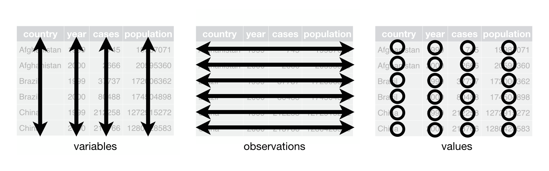
数据清洗是为了将数据中的无效部分去除,并最终整理成一个清晰的形式,方便接下来直接使用统计分析方法处理清洗后的数据。因此,需要知道 R 中大多数统计分析函数对于数据的形式有什么样的要求,即什么样的数据才是干净、整洁的。这里介绍 Tidyverse 提出的 tidy data 的概念,本质上是遵循“一人一行、一列一变量”的基本原则,tidydata 包括以下三条规则:
- 每一个变量都要有专属的一列(最重要);
- 每一份观察记录要有专属的一行;
- 每一个数据点要有专属的单元格。
- Tidy data 示例

- not tidy data 示例
tidy data,应该是这个样子:
所以,如何将数据整理成为 tidy data 的形式,通常也是 data cleaning 的一个环节。需要注意的是,不是说不整理成 tidy data 的形式就是错误的,而是说整理成这种形式更便于理解和统计分析。
16.1.3 Pipe operator
16.1.3.2 What is %>%
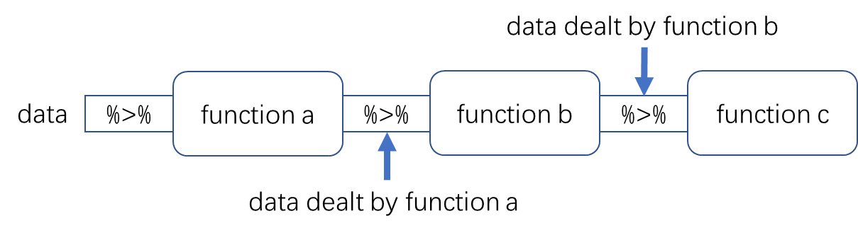
%>%的最基本用法是LHS %>% fun(...),本质上相当于fun(LHS, ...),即把LHS输送给fun,并默认作为第一个 argument,并且执行fun。
vec <- c(1, 2, 3)
vec %>% mean
#> [1] 2
mean(vec)#> [1] 216.1.3.3 Placeholder
当需要将%>%的LHS传递给右侧的fun,且不是作为首个 argument 时,就需要用到占位符(placeholder)了,与%>%匹配的 placeholder 是.。那么如何理解 placeholder?placeholder 就是先给以后要传递过来的LHS占个座,等LHS传过来了就它让作为这个位置的参数,然后执行fun。
df <- data.frame(x = c(1, 2, 3), y = c(4, 5, 6))
df %>%
  ncol %>%
  seq(from = 1, to = .)
#> [1] 1 2
16.1.3.4 why %>%
那既然是1:3 %>% mean与mean(1:3)是等价的,为什么要开发%>%?为了让代码看起来更加简洁易懂。
car_data <- transform(aggregate(
  . ~ cyl,
  data = subset(datasets::mtcars, hp > 100), # mtcars[mtcars$hp > 100, ]
  FUN = function(x) round(mean(x), 2)
), kpl = mpg*0.4251)
car_data要读懂上一段代码,首先要做的是根据()来判断到底哪部分先执行。可以看得出来,是先执行内层的aggregate(),再执行外层的transform()。除此自外,aggregate()的 argument 是 function 的执行结果,并且还是 function 套 function,这也增加了理解的难度。
car_data <-
  datasets::mtcars %>%
  subset(hp > 100) %>%
  aggregate(. ~ cyl, data = ., FUN = . %>% mean %>% round(2)) %>%  # the second dot is a placeholder, the 1st and 3rd ones are the dot notation of aggregate
  transform(kpl = mpg * 0.4251)
car_data使用%>%改写以后,就变成语义和结构上都更加清晰的一段代码,从上到下可以解读为:
- 将
mtcars中hp>100的部分取出; - 将上一步得到的数据使用
aggregate()按cyl分组求均值,结果取整,保留 2 位小数; - 将上一步得到的数据做 transformation,将
mpg这一列乘以0.4251,所得结果存新的一列kpl。
这样的代码读起来认知负担就远小于原始的代码。同时,从这个例子也可以看出来,%>%适合针对同一个 object 的序列操作。
16.1.3.5 Native pipe operator
随着 magrittr 包的影响力越来越大,使用%>%的人越来越多,R core team 也在 4.1.0 中加入了 native pipe operator ——|>,从此以后再也不用另外再加载 magrittr 包了。
那么|>和%>%有什么区别需要注意的吗?有,一共 8 点区别,其中前 4 点相对更常用
-
|>中右侧调用的 function 必须有明确的();
vec <- c(1, 2, 3)
vec %>% mean
#> [1] 2
vec %>% mean() # equivalent#> [1] 2
vec |> mean()#> [1] 2-
|>的 placeholder 是_;
df <- data.frame(x = c(1, 2, 3), y = c(4, 5, 6))
df %>%
  ncol %>%
  seq(from = 1, to = .)
#> [1] 1 2#> [1] 1 2-
|>中_必须用于有 name 的 argument;
letters[1:3] %>% paste(., collapse = " and ")#> [1] "a and b and c"#> Error in paste("_", collapse = " and "): pipe placeholder can only be used as a named argument (<input>:1:17)这就使得如果...在这种灵活且没有 name 的 argument 上使用_,需要取点巧
# use an name that is not used by any argument of paste
letters[1:3] |> paste(x = _, collapse = " and ")
#> [1] "a and b and c"
# use anonymous function
letters[1:3] |> (\(x) paste(x, collapse = " and "))()
#> [1] "a and b and c"- 一个
|>中的_只能在右侧使用一次;
letters[1:3] %>% paste(., .)#> [1] "a a" "b b" "c c"#> Error in paste(x = "_", y = "_"): pipe placeholder may only appear once (<input>:1:17)-
|>中_不允许在嵌套 function 中使用;
#> [1] 1.732051#> [1] 1.732051-
|>中_可以作为一系列 subsetting 的开头;
#> [1] -0.1351418#> [1] -0.1351418-
|>使用$时需要更加明确$是一个 function;
mtcars %>% `$`(cyl)#> [1] 6 6 4 6 8 6 8 4 4 6 6 8 8 8 8 8 8 4 4 4 4 8 8 8 8 4 4 4
#> [29] 8 6 8 4
mtcars |> (`$`)(cyl)#> [1] 6 6 4 6 8 6 8 4 4 6 6 8 8 8 8 8 8 4 4 4 4 8 8 8 8 4 4 4
#> [29] 8 6 8 4
mtcars |> base::`$`(cyl)#> [1] 6 6 4 6 8 6 8 4 4 6 6 8 8 8 8 8 8 4 4 4 4 8 8 8 8 4 4 4
#> [29] 8 6 8 4
fun <- `$`
mtcars |> fun(cyl)
#> [1] 6 6 4 6 8 6 8 4 4 6 6 8 8 8 8 8 8 4 4 4 4 8 8 8 8 4 4 4
#> [29] 8 6 8 4-
|>执行时不会生成额外的 environment。
x <- 1
"x" %>% assign(4)
x
#> [1] 1
# just like a function, %>% generates an additional
#   independent env when evaluating, everything therefore
#   happen in this environment, change will not be passed
#   to the parent environments
"x" |> assign(4)
x
#> [1] 4
# |> lead to direct assignment of x in the global
#   environment because no additional env.
"x" |> (\(y) assign(y, 3))()
x
#> [1] 4
#  anonymous function acts in a way similar to %>%,
#   since function call always generate additional env
What are the differences between R’s new native pipe |> and the magrittr pipe %>%?
16.2 Create data set
创建数据集指的是将收集来的数据创建为一个完整的数据集。根据具体情况的不同,可能有录入、合并等多种形式。
16.2.1 Import
采用线下回收纸质问卷的方式时,第一个要做的事就是人工将数据录入至电脑。这个过程中录入员非常容易因为数据量大、长时间录入而出现录入错误,所以一般会采取双人背对背录入同一批问卷数据的方式来交叉·核对。所以,这种场景下的任务目标就是对比两个数据集是否完全一致,如果不是,不一致的地方在哪里。
在开始对比之前,首先要保证两份数据集大体上的一致性,例如被试的数量、顺序,题目的数量、顺序、缺失数据的处理方式、是否有反向计分,等等。这些都是可以在录入之前就约定好采用相同的处理方式。
head(data_dirty_01)
head(data_dirty_02)- 是否完全一样
identical(data_dirty_01, data_dirty_02)#> [1] FALSE- 哪里不一样
如果两份数据文件记录的内容完全一样,但只是 element type 不同,identical()函数也会返回FALSE的结果,所以首先要检查是否存在 element type 上的不同。
# 判断是不是元素类型导致的问题
elem_type_data01 <- sapply(data_dirty_01, typeof)
elem_type_data01
#> gender ethnicity first_name last_name age
#> "integer" "integer" "character" "character" "integer"
#> P1 P2 P3 P4 P5
#> "double" "double" "double" "double" "double"
#> P6 P7 P8 P9 P10_att
#> "double" "double" "double" "double" "double"
#> P11 P12 P13 P14 P15
#> "double" "double" "double" "double" "double"
#> P16 W1 W2 W3 W4
#> "double" "double" "double" "double" "double"
#> W5 W6 W7 W8 W9
#> "double" "double" "double" "double" "double"
#> W10 W11 W12 W13 W14
#> "double" "double" "double" "double" "double"
#> W15 W16_att g1 g2 g3
#> "double" "double" "double" "double" "double"
#> g4 g5 g6 g7_att g8
#> "double" "double" "double" "double" "double"
#> g9 g10 g11 g12 g13
#> "double" "double" "double" "double" "double"
#> g14 g15 g16 S1 S2
#> "double" "double" "double" "double" "double"
#> S3 S4 S5 S6 S7
#> "double" "double" "double" "double" "double"
#> S8 S9 S10 S11 S12
#> "double" "double" "double" "double" "double"
#> S13_recode S14 S15 S16 J1
#> "double" "double" "double" "double" "double"
#> J2 J3 J4 J5 J6
#> "double" "double" "double" "double" "double"
#> J7 J8 J9 J10 J11
#> "double" "double" "double" "double" "double"
#> J12 J13 J14 J15 J16
#> "double" "double" "double" "double" "double"
#> time
#> "double"#> [1] TRUE确认了 element type 没有问题以后,就可以判断出来确实存在数据内容上的不同。接下来就是找到不同所在。
n_ob <- nrow(data_dirty_01)
locations <- which(data_dirty_01 != data_dirty_02, arr.ind = TRUE)
head(locations)
#> row col
#> [1,] 439 6
#> [2,] 614 6
#> [3,] 740 6
#> [4,] 904 6
#> [5,] 927 6
#> [6,] 972 6核对一下是不是不一样。
data_dirty_01[439, ]
data_dirty_02[439, ]16.2.2 Merge
当数据是分散在不同的设备,或者是数据是在不同的时间点采集时,往往会得到多份记录相同变量但具体数据信息不同的文件,此时就需要将多份文件合并成为一个完整的数据集。
- 不同被试相同变量
当只是针对不同被试测量了一次相同变量时,这样产生的多份数据只需要匹配变量的信息,即只需要将多份数据中相同的变量信息提取出来,然后纵向合并即可。
head(data_difsub_idevar_01)
head(data_difsub_idevar_02)
name_common_col <- intersect(names(data_difsub_idevar_01), names(data_difsub_idevar_02))
name_common_col
#> [1] "id" "humility"
#> [3] "egalitarian_belief" "stereotyping"
data_merged <-
rbind(
  data_difsub_idevar_01[name_common_col],
  data_difsub_idevar_02[name_common_col]
)
head(data_merged)- 相同被试不同变量
当针对同一批被试,测试了多次不同的变量,或者是在不同的时间点测量了相同的变量时,也可能产生多份数据文件,此时就需要以被试的背景信息为依据,来合并多份数据。
head(data_idesub_diffvar_01)
head(data_idesub_diffvar_02)使用merge()中的额外参数满足更多需求。
# the extra rows in x (data_idesub_diffvar_01) that are not in
#  y (data_idesub_diffvar_02) will be reserved
data_merged <- merge(data_idesub_diffvar_01, data_idesub_diffvar_02, all.x = TRUE)
tail(data_merged)
16.3 Convert into tidy data
创建完数据集以后,很有可能数据并不是 tidy data 的形式,大多是两种情况:
- Wider format: 一个变量的数据跨了好几列;
- Longer format: 一个观察记录跨了好几行。
上述两种情况都需要转换数据的形态,前者需要将数据从 wider format 转换成 longer format。在心理学领域的数据分析任务中,前者最为常见,所以本节只讲前者。
16.3.1 Wider to Longer
重复测量的数据是一个典型的 wider format。例如\(2\times2\)重复测量,实验处理一共是 4 个水平,但其实是把 A 和 B 这两个变量分在了 4 列。因此,需要执行 wider to longer 的转换,把 4 列的数据合并成 2 列,将原本的分组变量 A 和 B 分离出来,这就需要使用到 tidyr 包中的pivot_loger()。
# the most frequently used arguments of pivot_longer
pivot_longer(
  data,
  cols,
  names_to = "name",
  names_sep = NULL,
  names_pattern = NULL,
  values_to = "value"
)-
cols: 要转变为 longer format 的原 columns; -
names_to: 字符串向量,原 columns 的 names 将储存在新 column 的单元格里,新 column 的 name 由本参数设定。- 如果
names_to的长度大于 1,将会创建多个新的 columns。在这个情况下,必须提供names_sep或names_pattern来指定原 columns 的 names 怎么分配到新 columns 的单元格里去。-
NA:将会遗弃对应的新 column, -
.value:新 columns 的 names 是原 columns names 的一部分,新 columns 的单元格里储存对应的原 columns 单元格的数据,该参数会覆盖value_to参数的设定。
-
- 如果
-
names_sep: 指定原 columns names 的分割规则,既可以是 numeric vector,表示按照位置来分割,也可以是单个字符(类似read.table()中的sep参数,可以是正常的字符,如"_",也可以是正则表达式,如"\.")。 -
names_pattern: 正则表达式,原 columns 的 names 将按照该表达式的匹配结果分割并创建新 columns。 -
values_to: 字符,原 column 的单元格中的数据将单独储存在一个新 column (value column)里,新 value column 的 name 由本参数设定。如果names_to中包含了.value(必须给定names_sep或names_pattern),本参数的设定会被忽略,并且新 value column 的 name 来自原 columns name 中的指定部分。
- 基本用法:4 个必写参数,
pivot(data, cols, names_to, values_to)
data_virtual_imaginary <- read.table(
  "F:/Nutstore backup/R/codes/RBA/data/untidy data virtual imaginary.txt"
)
head(data_virtual_imaginary)
data_virtual_imaginary |>
  t() |>
  as.data.frame(row.names = 1:ncol(data_virtual_imaginary)) |>
  cbind(participant = LETTERS[1:ncol(data_virtual_imaginary)]) |>
  pivot_longer(
    cols = c("virtual_imaginary", "no_virtual_imaginary"),
    names_to = "group",
    values_to = "count"
  ) |>
dplyr::select(participant, group, count)- 额外参数:
names_sep
# numeric
head(data_repeated_2f)
data_repeated_2f |>
  pivot_longer(
    cols = 2:7,
    names_to = c("A", "B"),
    names_sep = 2,
    values_to = "score"
  )
# single string
data_repeated_2f_underline <- data_repeated_2f
names(data_repeated_2f_underline)[2:7] <- c("A1_B1", "A2_B1", "A1_B2", "A2_B2", "A1_B3", "A2_B3")
head(data_repeated_2f_underline)
data_repeated_2f_underline |>
  pivot_longer(
    cols = 2:7,
    names_to = c("A", "B"),
    names_sep = "_",
    values_to = "score"
)- 额外参数:
names_pattern
head(data_repeated_2f)
data_repeated_2f |>
  pivot_longer(
    cols = 2:7,
    names_to = c("A", "B"),
    names_pattern = "([A-Z][0-9])([A-Z][0-9])",
    values_to = "score"
)-
names_to的特殊用法
-
NA: will discard the corresponding component of the column name.
head(data_repeated_2f)
data_repeated_2f |>
  pivot_longer(
    cols = 2:7,
    names_to = c(NA, "B"),
    names_pattern = "([A-Z][0-9])([A-Z][0-9])",
    values_to = "score"
)-
.value: indicates that the corresponding component of the column name defines the name of the output column containing the cell values, overridingvalues_toentirely.
data_partipipant_id_in_col <-
  sapply(1:9, \(x) sample(5, size = 3, replace = T)) |>
  as.data.frame() |>
  setNames(c(
    "var1_t1", "var2_t1", "var3_t1",
    "var1_t2", "var2_t2", "var3_t2",
    "var1_t3", "var2_t3", "var3_t3"
  ))
data_partipipant_id_in_col
# component of the column name (i.e. "VAR1") defines the name of the output column
data_partipipant_id_in_col |>
  pivot_longer(
    cols = 1:ncol(data_partipipant_id_in_col),
    names_to = c(".value", "time_point"),
    names_sep = "_"
)更多关于pivot_longer()的高级用法详见vignette("pivot")。
16.4 Reverse coding
Reverse coding is a technique frequently used in survey study.
16.4.1 What is reverse coding
One common validation technique for survey items is to rephrase a “positive” item in a “negative” way. When done properly, this can be used to check if respondents are giving consistent answers.
For example, consider the following two items concerning “extraversion”:
- I see myself as someone who is talkative.
- Disagree strongly
- Disagree a little
- Neither agree nor disagree
- Agree a little
- Agree strongly
- I see myself as someone who tends to be quiet.
- Disagree strongly
- Disagree a little
- Neither agree nor disagree
- Agree a little
- Agree strongly
For question 1, “agree strongly” corresponds to the “most extraverted” option, and “disagree strongly” corresponds to the “least extraverted” option. However, for question 2, “disagree strongly” corresponds to the “most extraverted” option, and “agree strongly” corresponds to the “least extraverted” option. We say that question 2 is reverse-coded.
16.4.2 How to do reverse coding
Manually recode.
df <- data.frame(x = sample(5, size = 10, replace = TRUE))
df
df[df == 1] <- 50
df[df == 2] <- 40
df[df == 3] <- 30
df[df == 4] <- 20
df[df == 5] <- 10
df <- df/10
df
Since recoding Likert scale survey data are repeat operations, they can be converted into a for loop,
df <- data.frame(x = sample(5, size = 10, replace = TRUE))
df
scale_piont <- 5
coding_rule <- seq(scale_piont*10, 10, by = -10)
for (i in 1:scale_piont) {
  df[df == i] <- coding_rule[i]
}
df <- df/10
df
What is its apply()/sapply()/lapply() substitute?
df <- data.frame(x = sample(5, size = 10, replace = TRUE))
scale_piont <- 5
coding_rule <- seq(scale_piont*10, 10, by = -10)
# sapply(1:scale_piont, \(x) {
#   df[df == x] <<- coding_rule[x]
#   return(NULL)
# })
# df <- df / 10
# a more straightforward solution by Shusheng Liu
df <- sapply(df, \(i)coding_rule[i])/10
The code above illustrates the basic idea of recoding. However, a more flexible function is available, and reinventing the wheel is not recommended
recode(var, recodes)
-
var: numeric vector, character vector, or factor. -
recodes: character string of recode specifications: see below.
Recode specifications appear in a character string, separated by default by semicolons (see the examples below), each of the form input=output.
Several recode specifications are supported:
- single value: For example,
0=NA. - vector of values: For example,
c(7, 8, 9) = "high". - range of values: For example,
7:9 = "C". Note::is not the R sequence operator. In addition, you may not use:with thecfunction within a recode specification, so for examplec(1, 3, 5:7)will cause an error. The:is the default value of therecode intervaloperator; a non-default value may be specified. -
else: everything that does not fit a previous specification. For example,else = NA. Note thatelsematches all otherwise unspecified values on input, includingNA, and if present should appear last among the recode specifications.
Character data and factor levels on the left-hand side of a recode specification must be quoted. Thus, e.g., c(a, b, c) = "low" is not allowed, and should be c("a", "b", "c") = "low". Similarly, the colon is reserved for numeric data, and, e.g., c("a":"c") = "low" is not allowed. If the var argument is a character variable with (some) values that are character representations of numbers, or a factor with (some) levels that are numbers (e.g., "12" or "-2"), then these too must be quoted and cannot be used with colons (e.g., "15":"19" = "15 to 19" is not allowed, and could be specified as c("15", "16", "17", "18", "19") = "15 to 19", assuming that all values are the character representation of whole numbers).
x <- rep(1:3, times = 3)
x
#> [1] 1 2 3 1 2 3 1 2 3
car::recode(x, 'c(1, 2) = "A"; else = "B"')#> [1] "A" "A" "B" "A" "A" "B" "A" "A" "B"
# don't miss the double quote if recode numeric into character or vice versa
#   otherwise error
car::recode(x, "c(1, 2) = A; else = B")
#> Error in car::recode(x, "c(1, 2) = A; else = B"):
#> in recode term: else = B
#> message: Error in eval(parse(text = strsplit(term, to.value)[[1]][2])) :
#> object 'B' not foundReverse-code a Liker-5 point variable.
df <-
  data.frame(
    x = sample(5, size = 10, replace = TRUE),
    y = sample(5, size = 10, replace = TRUE)
  )
df$x
#> [1] 1 5 1 4 5 5 3 5 1 3
# reverse code x
df$x <- car::recode(df$x, recodes = "1=5;2=4;3=3;4=2;5=1")
df$x
#> [1] 5 1 5 2 1 1 3 1 5 3
# generate recode specifications with paste
# df$x <- car::recode(df$x, paste(1:5, 5:1, sep = "=", collapse = ";"))
# df < df - 6 # By Yuchen Liu, effective by less flexible than recode
Reverse-code multiple variables simultaneously with a self-defined function.
# author: Wenzheng Lin
# collaborator: Yujun Li
recode_vars <- function(
    data,
    max = 5,
    min = 1,
    vars = names(data)
  ){
  rule <- paste(min:max, max:min, sep = "=", collapse = ";")
  if (!is.data.frame(data) & is.vector(data)) {
    # recode single variable
    output <- car::recode(data, rule)
    return(output)
  }
  output <- as.data.frame(apply(data[vars], 2, \(x) car::recode(x, rule)))
  # recode some variables
  if (ncol(data) != length(vars)) {
    vars_rest <- !names(data) %in% vars
    output <- data.frame(data[, vars_rest], output)
    names(output)[1:(ncol(output) - length(vars))] <- names(data)[vars_rest]
    output <- output[names(data)]
  }
  return(output)
}
df <-
  data.frame(
    x = sample(7, size = 10, replace = TRUE),
    y = sample(7, size = 10, replace = TRUE),
    z = sample(7, size = 10, replace = TRUE)
  )
head(df)
df_recode_all <- recode_vars(df, max = 7)
head(df_recode_all)
16.5 Aberrant response
Aberrant response 的种类很多,常见的如下:
- Validity measure/attention check,
- Quantitative unrealistic response,
- Speedness,
- Repeated observations,
- Recursive responses,
- Outlier,
- Missing data.
处理 aberrant response 的核心是通过一些特定的操作产生一个 logical object,TRUE可以表示是 aberrant response,FALSE则相反。再使用该 logical object 作为 subsetting 的 index 就可以提取出找到的所有 aberrant response,至于找出来以后是直接删除还是另作处理就很简单了。
16.5.1 Validity measure/attention check, unrealistic response, speedness
这三类都适用相同的处理办法,即使用 relational + logical operators 的方式生成 logical object 作为 index,然后使用该 index 来 subsetting 即可。
16.5.1.1 Validity measure/attention check
Too Good to Be True: Bots and Bad Data From Mechanical Turk
The attention checks consisted of the following:
- embedded on the Grit scale—“Select‘Somewhat like me’ for this statement,”
- embedded on the Beck Depression Inventory—“1 – Select this option,” and
- embedded on the Borderline Personality Inventory—“Select ‘Yes’ for this statement.”
A more detailed introduction on attention check: Prolific’s Attention and Comprehension Check Policy
df <- data.frame(
  x = sample(
    1:5,
    size = 10,
    replace = TRUE,
    prob = c(0.6, 0.1, 0.1, 0.1, 0.1)
  ),
  y = sample(5, size = 10, replace = TRUE),
  z = sample(5, size = 10, replace = TRUE)
)
head(df)
# assume x is the attention check item and participant is requested to select 1.
id_fail_atten_check <- (1:nrow(df))[df$x != 1]
id_fail_atten_check
#> [1] 2 4 5
df_filtered <- df[-id_fail_atten_check, ]16.5.1.2 Quantitative unrealistic response
需要根据问卷的具体内容来判断到底什么样的作答才算 unrealistic。例如询问被试的日均手机使用时间,有人填了 25 小时,或者是同一份问卷内有多个询问手机使用时间的题目,结果被试在这些题目上填写的使用时间加起来大于 24 小时,显然就是 unrealistic。针对这种可以使用一定数值标准(例如>24)为依据判断作答是否 unrealistic 的情况,称之为 quantitative unrealistic response。文本类型的 qualitative unrealistic response 则需要人工检查。
16.5.2 Repeated observations
有些时候可能由于人工录入数据的时候,出现了同一份问卷录入了两次甚至更多的问题,此时就产生了 repeated observations,使用duplicated()检测。
df <- data.frame(
  x = sample(
    1:5,
    size = 10,
    replace = TRUE,
    prob = c(0.6, 0.1, 0.1, 0.1, 0.1)
  ),
  y = sample(5, size = 10, replace = TRUE),
  z = sample(5, size = 10, replace = TRUE)
)
head(df)
id_dup_row <- duplicated(df)
id_dup_row
#> [1] FALSE FALSE FALSE FALSE FALSE TRUE TRUE FALSE TRUE
#> [10] FALSE TRUE TRUE FALSE TRUE TRUE
df[!id_dup_row, ]16.5.3 Recursive responses
当问卷总题数较长且被试失去了兴趣和耐心时,被试很有可能会出现低动机(low motivation)的状况,并最终驱动 ta 开始随意作答,出现规律性的重复作答,如 345345345。但是这种情况的处理是有争议的,一般建议在没有非常强的证据时(如伴随有异常短的 response time),不将类似的作答作为 aberrant response。因为无法排除是正常作答的被试选择了类似 345345345345 的 recursive responses 的可能。因此,更建议的做法是找出有 recursive response 的被试,然后结合这些被试在每一题上的 response time 来 double check。
- locate recursive responses
可选方案:使用paste()将所有作答横向拼接为字符串,然后使用grep()查找指定模式的 recursive responses。
head(df_all)#> [1] "15333455135224134242" "33441211352151425253"
#> [3] "34314513123123123123" "54135515323255122215"
#> [5] "23442221545312132222" "21123234522122311521"
#> [7] "54223253243222354245" "31232545251315331345"
#> [9] "53345325211315212554" "35142143132234442214"
grep("123123123123", df_char)#> [1] 3- check response time
可选方案,t test (more informative) or Kolmogorov-Smirnov Tests.
df_char <- apply(df_all[, 1:20], 1, \(x) paste(x, collapse = ""))
id_recur_res <- grep("123123123123", df_char)
results_match <- regexec("123123123123", df_char)
start_recur_res <- results_match[[3]][1] + 20
end_recur_res <- start_recur_res + attributes(results_match[[3]])$match.length - 1
rt_normal_res <- df_all[id_recur_res, 21:(start_recur_res - 1)]
rt_recur_res <- df_all[id_recur_res, start_recur_res:end_recur_res]
t.test(rt_normal_res, rt_recur_res)
#>
#> Welch Two Sample t-test
#>
#> data: rt_normal_res and rt_recur_res
#> t = 4.8974, df = 7.0046, p-value = 0.001755
#> alternative hypothesis: true difference in means is not equal to 0
#> 95 percent confidence interval:
#> 4891.772 14023.452
#> sample estimates:
#> mean of x mean of y
#> 9793.6742 336.0622
ks.test(as.numeric(rt_recur_res), as.numeric(rt_normal_res))#>
#> Exact two-sample Kolmogorov-Smirnov test
#>
#> data: as.numeric(rt_recur_res) and as.numeric(rt_normal_res)
#> D = 1, p-value = 1.588e-05
#> alternative hypothesis: two-sided16.5.4 Outlier
Outliers in statistics are considered as the data values which differ considerably from the bulk of a given data set. Outliers can strongly bias statistical inference.
cor_matrix <- matrix(c(1, 0, 0, 1), nrow = 2, ncol = 2)
data <- MASS::mvrnorm(1000, mu = rep(0, 2), Sigma = cor_matrix)
plot(data)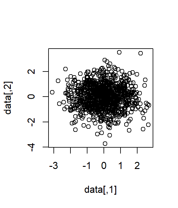
cor.test(data[, 1], data[, 2])#>
#> Pearson's product-moment correlation
#>
#> data: data[, 1] and data[, 2]
#> t = -0.35719, df = 998, p-value = 0.721
#> alternative hypothesis: true correlation is not equal to 0
#> 95 percent confidence interval:
#> -0.07324757 0.05072280
#> sample estimates:
#> cor
#> -0.01130583
# add_outliers
n_outlier <- 20
id_outlier <- order(rowSums(data), decreasing = T)[1:n_outlier]
data[id_outlier, ] <- data[id_outlier, ] + matrix(
  runif(n_outlier * 2, 2, 3),
  nrow = n_outlier, ncol = 2
)
plot(data)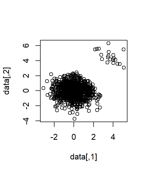
cor.test(data[, 1], data[, 2])#>
#> Pearson's product-moment correlation
#>
#> data: data[, 1] and data[, 2]
#> t = 6.8605, df = 998, p-value = 1.203e-11
#> alternative hypothesis: true correlation is not equal to 0
#> 95 percent confidence interval:
#> 0.1522271 0.2706498
#> sample estimates:
#> cor
#> 0.212217416.5.4.1 Mahalanobis Distance
\[D^2_i=(\boldsymbol{x}_i-\boldsymbol{\hat{\mu}})'\boldsymbol{S}^{-1}(\boldsymbol{x}_i-\boldsymbol{\hat{\mu}}).\]
\(D^2\) theoretically follows a \(\chi^2\) distribution with degrees of freedom (\(df\)) equal to the number of variables.
dis_mh <- mahalanobis(data, center = colMeans(data), cov = cov(data))
id_outlier_mh <- which(dis_mh > qchisq(p = 1 - 0.05, df = ncol(data)))
id_outlier_mh
#> [1] 22 68 76 84 120 151 172 185 205 207 243 247 266 267
#> [15] 270 271 297 310 327 347 360 370 397 403 420 425 432 482
#> [29] 489 493 504 579 627 672 702 705 745 813 829 832 868 905
#> [43] 943
id_outlier %in% id_outlier_mh#> [1] TRUE TRUE TRUE TRUE TRUE TRUE TRUE TRUE TRUE TRUE TRUE
#> [12] TRUE TRUE TRUE TRUE TRUE TRUE TRUE TRUE TRUE
cor.test(data[-id_outlier_mh, 1], data[-id_outlier_mh, 2])#>
#> Pearson's product-moment correlation
#>
#> data: data[-id_outlier_mh, 1] and data[-id_outlier_mh, 2]
#> t = -0.40694, df = 955, p-value = 0.6841
#> alternative hypothesis: true correlation is not equal to 0
#> 95 percent confidence interval:
#> -0.07647432 0.05024608
#> sample estimates:
#> cor
#> -0.0131669916.5.4.2 Minimum Covariance Determinant
It is clearly that Mahalanobis distance has an inflated type-I error rate, since it detects more than 20 outliers in the previous example. This is because Mahalanobis distance uses the mean vector and covariance matrix, which already contain considerable amount of bias due to outliers. It makes more sense to use more accuratly estimated mean and covariance when calculating Mahalanobis distance. This is the idea behind Minimum Covariance Determinant, which calculates the mean and covariance matrix based on the most central subset of the data.
mean_cov_75 <- MASS::cov.mcd(data, quantile.used = nrow(data)*.75)
mh_75 <- mahalanobis(data, mean_cov_75$center, mean_cov_75$cov)
id_outlier_mh_75 <- which(mh_75 > qchisq(p = 1 - 0.05, df = ncol(data)))
id_outlier_mh_75
#> [1] 22 25 56 65 68 76 84 94 120 136 146 151 172 178
#> [15] 185 204 205 207 213 215 243 247 250 266 267 270 271 272
#> [29] 297 310 327 347 360 370 397 403 420 425 432 446 448 478
#> [43] 482 489 493 504 533 579 627 635 672 702 705 745 774 792
#> [57] 798 813 829 832 868 877 900 905 943 955 963 973 990
id_outlier %in% id_outlier_mh_75#> [1] TRUE TRUE TRUE TRUE TRUE TRUE TRUE TRUE TRUE TRUE TRUE
#> [12] TRUE TRUE TRUE TRUE TRUE TRUE TRUE TRUE TRUE
cor.test(data[-id_outlier_mh_75, 1], data[-id_outlier_mh_75, 2])#>
#> Pearson's product-moment correlation
#>
#> data: data[-id_outlier_mh_75, 1] and data[-id_outlier_mh_75, 2]
#> t = -0.93584, df = 929, p-value = 0.3496
#> alternative hypothesis: true correlation is not equal to 0
#> 95 percent confidence interval:
#> -0.09475286 0.03362729
#> sample estimates:
#> cor
#> -0.03068936Although the type I error rate of MCD-based Mahalanobis distance is still inflated, it performs arguably better than the traditional one. Methods to deal with outliers abound, and none of them is perfect. Interested readers in more details about how to detect outliers are refered to Leys et al. (2018).
Leys, C., Klein, O., Dominicy, Y., & Ley, C. (2018). Detecting multivariate outliers: Use a robust variant of Mahalanobis distance. Journal of Experimental Social Psychology, 74, 150-156.