Chapter 33 use county names from health data
national_health_merged <- natl_health_data_cty %>%
  right_join(us_counties, by = c("fips" = "GEOID")) |>
  rename(county = county.x)
Now map
national_health_merged %>%
  select(fips, county, average_number_of_mentally_unhealthy_days, geometry) |>
    ggplot(aes(fill = average_number_of_mentally_unhealthy_days)) +
    geom_sf(aes(geometry = geometry), color = NA) +
    scale_fill_viridis_c(option = "viridis",
            name = "Average \nMentally \nUnhealthy \nDays") +
    labs(title = "Average Mentally Unhealthy Days by County",
          subtitle = "US, 2025 Health Data Estimates") +
    theme_void() # Removes axes and grid lines for a cleaner map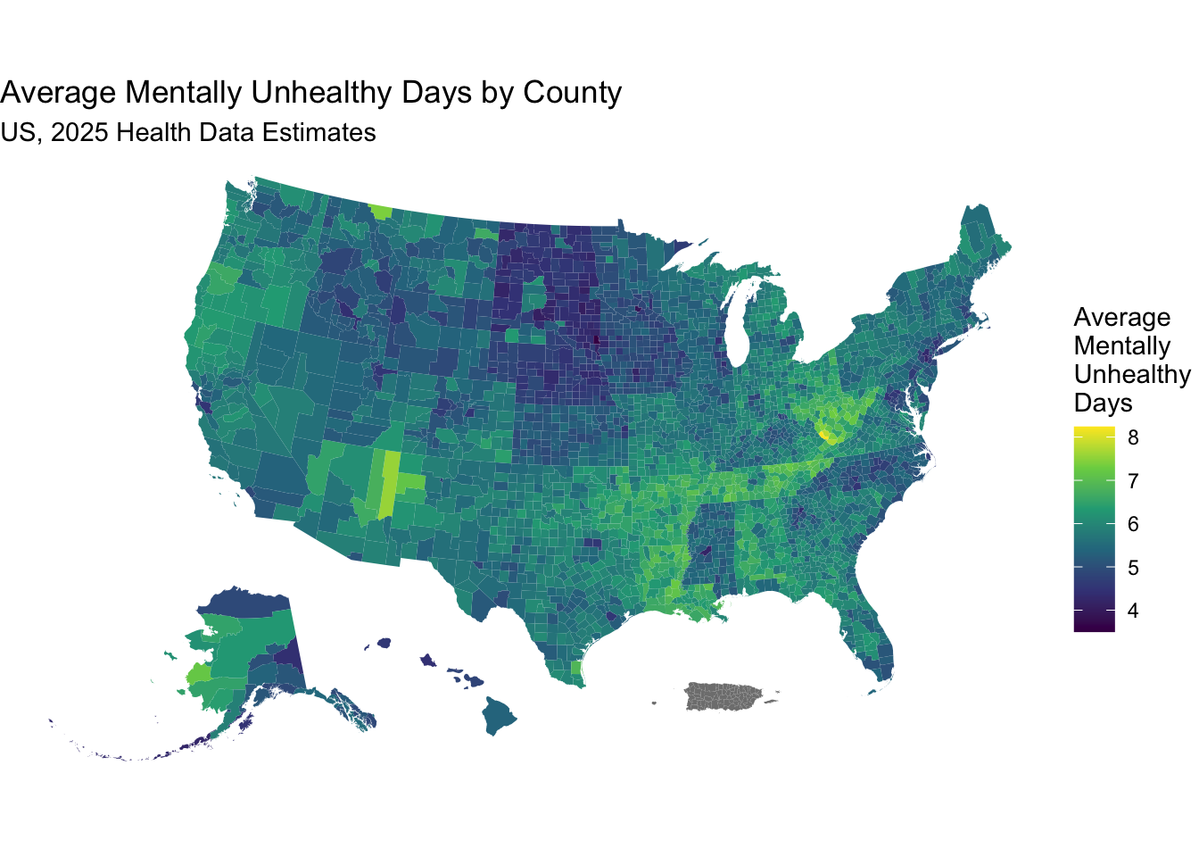
33.1 Mapping Distances
Acute illness and trauma from MVI (motor vehicle injury) is a major cause of death and disability in the US, and is a major public health problem. Outcomes are influenced by distance/time from specialty care. Using {mapboxapi} and the {tigris} package, we can map distances from a set of census tracs to a hospital at a given location, which can serve as a measure of time to travel to reach specialty care.
library(mapboxapi)
library(tigris)
library(tidyverse)
library(sf)
library(crsuggest)
# Set up Mapbox API key
# You need to set up a Mapbox account and get an API key
# see https://docs.mapbox.com/help/getting-started/access-tokens/
# and then store this token in your .Renviron file as MAPBOX_API_KEY
# mapbox_key <- Sys.getenv("MAPBOX_API_KEY")
# mb_access_token(mapbox_key, install = TRUE) # run this once

# Load Census tracts for the state of Michigan using (tigris)

mi_tracts <-
  tracts(state = "MI", cb = TRUE) %>%
  st_transform(2163) # a coordinate reference system transformation
## Retrieving data for the year 2022# Find the right coordinate system to use; in this case we'll use 26990
mi_crs <- suggest_top_crs(mi_tracts, units = "m")## Using the projected CRS NAD27 / UTM zone 15N which uses 'm' for measurement units. Please visit https://spatialreference.org/ref/epsg/26715/ for more information about this CRS.# Get the location of the University of Michigan hospital in Ann Arbor, Michigan
#
# You can use the mb_geocode() function to get the coordinates of a location
hospital_location <- mb_geocode("University of Michigan Hospital, Ann Arbor, MI")
# Use mb_matrix() to calculate driving time from all Michigan Census tracts to the hospital
# mi_tracts_points <- mi_tracts %>%
# st_transform(mi_crs) %>%
# erase_water(area_threshold = 0.95) %>% # can't drive through lakes
# st_point_on_surface()
# Now get driving time to the hospital from each tract
# Takes a few minutes to map driving times
# by default uses the centroid of each census tract as origin point
time_to_hospital <- mb_matrix(
origins = mi_tracts,
destinations = hospital_location
) %>%
as.vector()## Splitting your matrix request into smaller chunks and re-assembling the result.## Using feature centroids for origins## ■■ 2% | ETA: 1m## ■■ 5% | ETA: 2m## ■■■ 7% | ETA: 2m## ■■■■ 10% | ETA: 2m## ■■■■■ 12% | ETA: 2m## ■■■■■ 15% | ETA: 2m## ■■■■■■ 16% | ETA: 2m## ■■■■■■■ 19% | ETA: 2m## ■■■■■■■ 21% | ETA: 2m## ■■■■■■■■ 23% | ETA: 2m## ■■■■■■■■■ 26% | ETA: 2m## ■■■■■■■■■ 28% | ETA: 2m## ■■■■■■■■■■ 30% | ETA: 1m## ■■■■■■■■■■■ 32% | ETA: 1m## ■■■■■■■■■■■ 35% | ETA: 1m## ■■■■■■■■■■■■ 37% | ETA: 1m## ■■■■■■■■■■■■■ 40% | ETA: 1m## ■■■■■■■■■■■■■■ 42% | ETA: 1m## ■■■■■■■■■■■■■■ 44% | ETA: 1m## ■■■■■■■■■■■■■■■ 46% | ETA: 1m## ■■■■■■■■■■■■■■■■ 48% | ETA: 1m## ■■■■■■■■■■■■■■■■ 51% | ETA: 1m## ■■■■■■■■■■■■■■■■■ 53% | ETA: 1m## ■■■■■■■■■■■■■■■■■■ 56% | ETA: 1m## ■■■■■■■■■■■■■■■■■■ 58% | ETA: 1m## ■■■■■■■■■■■■■■■■■■■ 60% | ETA: 1m## ■■■■■■■■■■■■■■■■■■■■ 62% | ETA: 49s## ■■■■■■■■■■■■■■■■■■■■ 65% | ETA: 46s## ■■■■■■■■■■■■■■■■■■■■■ 67% | ETA: 43s## ■■■■■■■■■■■■■■■■■■■■■■ 69% | ETA: 40s## ■■■■■■■■■■■■■■■■■■■■■■■ 72% | ETA: 37s## ■■■■■■■■■■■■■■■■■■■■■■■ 74% | ETA: 33s## ■■■■■■■■■■■■■■■■■■■■■■■■ 76% | ETA: 31s## ■■■■■■■■■■■■■■■■■■■■■■■■ 78% | ETA: 28s## ■■■■■■■■■■■■■■■■■■■■■■■■■ 81% | ETA: 25s## ■■■■■■■■■■■■■■■■■■■■■■■■■■ 83% | ETA: 22s## ■■■■■■■■■■■■■■■■■■■■■■■■■■■ 85% | ETA: 19s## ■■■■■■■■■■■■■■■■■■■■■■■■■■■ 88% | ETA: 16s## ■■■■■■■■■■■■■■■■■■■■■■■■■■■■ 90% | ETA: 14s## ■■■■■■■■■■■■■■■■■■■■■■■■■■■■■ 92% | ETA: 10s## ■■■■■■■■■■■■■■■■■■■■■■■■■■■■■ 94% | ETA: 7s## ■■■■■■■■■■■■■■■■■■■■■■■■■■■■■■ 97% | ETA: 4s## ■■■■■■■■■■■■■■■■■■■■■■■■■■■■■■■ 99% | ETA: 1s# Add the driving time to the Census tracts data
mi_tracts$time_to_hospital <- time_to_hospital
mi_tracts$time_to_hospital <- as.numeric(mi_tracts$time_to_hospital)
# Remove any NA values (if any)
#mi_tracts <- mi_tracts %>%
#filter(!is.na(time_to_hospital))
# Visualize the driving time to the hospital using ggplot2
ggplot(mi_tracts, aes(fill = time_to_hospital)) +
geom_sf(color = "black") +
scale_fill_viridis_c(option = "viridis", name = "Driving Time (minutes)") +
labs(
title = "Driving Time to The University of Michigan Hospital",
subtitle = "From Individual Census Tracts in Michigan",
caption = "Data source: Mapbox Directions API"
) +
theme_void() +
coord_sf(crs = mi_crs)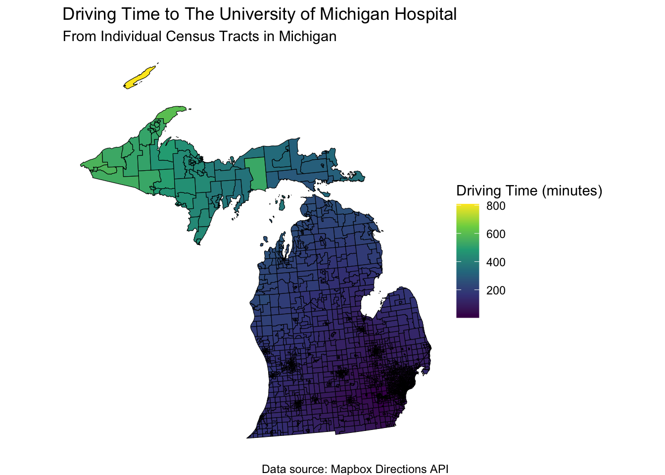
33.2 We can narrow this down to a smaller Area, such as Philadelphia, and driving time to the Children’s Hospital of Philadelphia (CHOP).
When your child is sick, you might want to race them to the local Children’s Hospital. How long will it take?
## Retrieving data for the year 2022chop <- mb_geocode("Children's Hospital of Philadelphia, Philadelphia, PA")
# takes about 40 seconds
time_to_chop <- mb_matrix(
origins = philly_tracts,
destinations = chop) %>%
as.vector()## Splitting your matrix request into smaller chunks and re-assembling the result.## Using feature centroids for origins## ■■■■■ 12% | ETA: 8s## ■■■■■■■■ 24% | ETA: 11s## ■■■■■■■■■■■■■ 41% | ETA: 9s## ■■■■■■■■■■■■■■■■■■■ 59% | ETA: 7s## ■■■■■■■■■■■■■■■■■■■■■■■■ 76% | ETA: 4s## ■■■■■■■■■■■■■■■■■■■■■■■■■■■■■ 94% | ETA: 1sphilly_tracts$time_to_chop <- time_to_chop
ggplot(philly_tracts, aes(fill = time_to_chop)) +
geom_sf(color = "black") +
scale_fill_viridis_c(option = "viridis", name = "Driving Time (minutes)") +
labs(
title = "Driving Time to The Children's Hospital of Philadelphia",
subtitle = "From Individual Census Tracts in Philadelphia",
caption = "Data source: Mapbox Directions API"
) +
theme_void()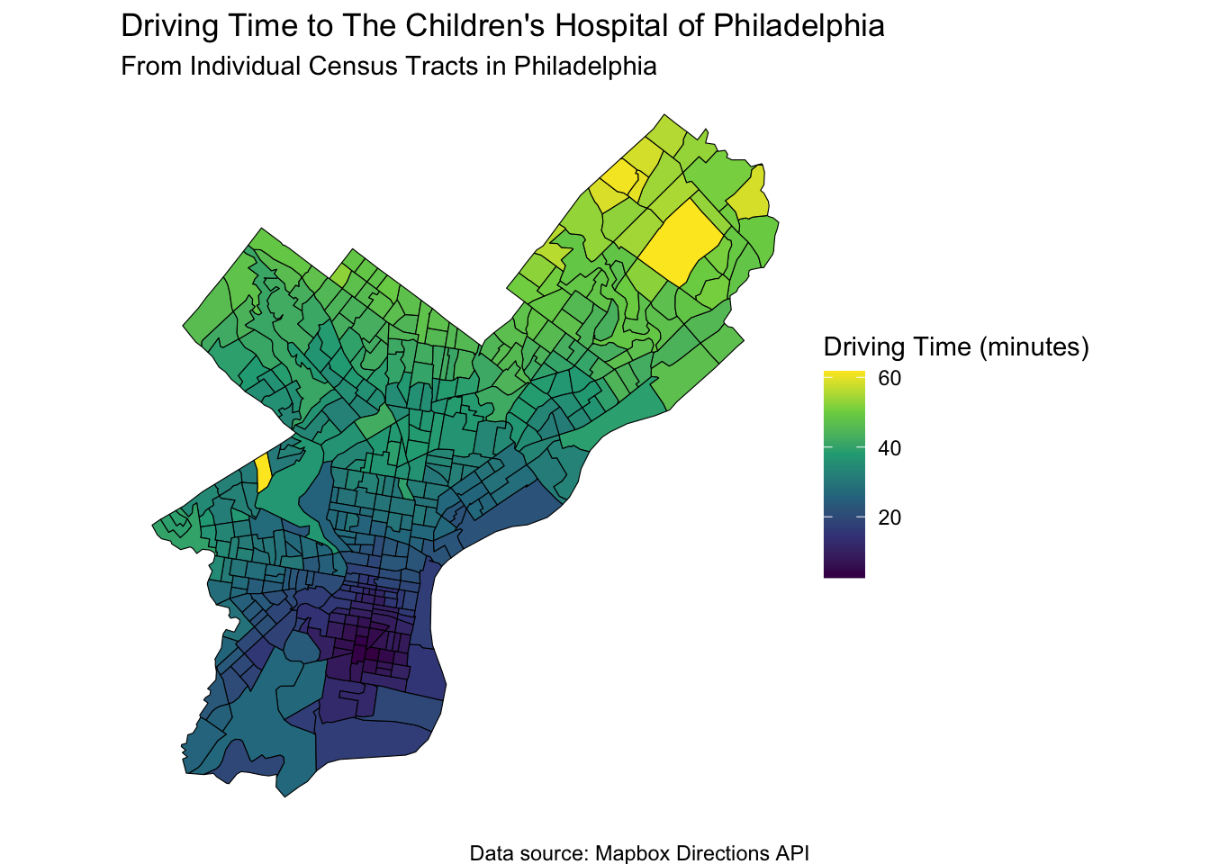
This is not the only way to map distances, but it is a good way to get started.
You can use the Google Distance API via the {googleway} package, or the {osrm} package to access the Open Source Routing Machine, which is a free routing service that uses OpenStreetMap data.
There is the R5 routing engine, which is a free routing service that uses OpenStreetMap data, and the {r5r} package to access it.
There is the Valhalla routing engine, which is a free routing service that uses OpenStreetMap data, and the {valhallar} package to access it.
The Mapbox and Google options are great for smaller jobs as they are very quick to set up once you have an API key and they have traffic built-in. But be careful - they can get expensive quickly if you are mapping thousands of individual addresses. Mapbox limits you to 100K free geocodes per month. Google limits you to a maximum of 25 origins or 25 destinations per request, and a rate limit of 3000 elements (origins * destinations) per minute.
For bigger jobs, look to r5r and Valhalla - both based on open-source engines.
While these tools are more challenging to set up than using an API, they are well worth it for batch jobs.
Valhalla in particular can be tricky to set up; it may be best used with Docker.
There are lots of great resources in this space.
33.3 Driving to UCLA Reagan Hospital
If you are living in the traffic jam that makes up the 5 county Los Angeles metro area, you might want to know how long it will take to get to the UCLA Reagan Hospital in Westwood.
library(mapboxapi)
library(tidyverse)
library(tigris)
library(sf)
library(crsuggest)
# Set up Mapbox API key
# You need to set up a Mapbox account and get an API key
# see https://docs.mapbox.com/help/getting-started/access-tokens/
# and then store this token in your .Renviron file as MAPBOX_API_KEY
# mb_access_token(Sys.getenv("MAPBOX_API_KEY"), install = TRUE)

# Load Census tracts for the Los Angeles metro area using (tigris)
# Note that this will take a few minutes to run

la_tracts <-
  tracts(state = "CA", county = c("Los Angeles", "Orange",
      "Riverside", "San Bernardino", "Ventura"), cb = TRUE) %>%
  st_transform(26910) # a coordinate reference system transformation
## Retrieving data for the year 2022# Find the right coordinate system to use; in this case we'll use 26910
la_crs <- suggest_top_crs(la_tracts, units = "m")## Using the projected CRS NAD83 / California zone 6 which uses 'm' for measurement units. Please visit https://spatialreference.org/ref/epsg/26946/ for more information about this CRS.# Get the location of the UCLA Reagan Hospital in Westwood, Los Angeles, California
hospital_location <- mb_geocode("UCLA Ronald Reagan Medical Center, Los Angeles, CA")
# Use mb_matrix() to calculate driving time from all Los Angeles metro Census tracts to the hospital - about 4 minutes
time_to_hospital <- mb_matrix(
origins = la_tracts,
destinations = hospital_location
) %>%
as.vector()## Splitting your matrix request into smaller chunks and re-assembling the result.## Using feature centroids for origins## ■■ 2% | ETA: 2m## ■■ 4% | ETA: 3m## ■■■ 6% | ETA: 3m## ■■■ 7% | ETA: 3m## ■■■■ 9% | ETA: 3m## ■■■■ 11% | ETA: 3m## ■■■■■ 12% | ETA: 3m## ■■■■■ 13% | ETA: 3m## ■■■■■■ 15% | ETA: 3m## ■■■■■■ 17% | ETA: 3m## ■■■■■■■ 18% | ETA: 2m## ■■■■■■■ 20% | ETA: 2m## ■■■■■■■ 21% | ETA: 2m## ■■■■■■■■ 23% | ETA: 2m## ■■■■■■■■ 25% | ETA: 2m## ■■■■■■■■■ 26% | ETA: 2m## ■■■■■■■■■ 28% | ETA: 2m## ■■■■■■■■■■ 30% | ETA: 2m## ■■■■■■■■■■ 31% | ETA: 2m## ■■■■■■■■■■■ 32% | ETA: 2m## ■■■■■■■■■■■ 34% | ETA: 2m## ■■■■■■■■■■■■ 36% | ETA: 2m## ■■■■■■■■■■■■ 37% | ETA: 2m## ■■■■■■■■■■■■■ 39% | ETA: 2m## ■■■■■■■■■■■■■ 41% | ETA: 2m## ■■■■■■■■■■■■■■ 42% | ETA: 2m## ■■■■■■■■■■■■■■ 44% | ETA: 2m## ■■■■■■■■■■■■■■■ 45% | ETA: 2m## ■■■■■■■■■■■■■■■ 47% | ETA: 2m## ■■■■■■■■■■■■■■■■ 49% | ETA: 2m## ■■■■■■■■■■■■■■■■ 50% | ETA: 2m## ■■■■■■■■■■■■■■■■■ 52% | ETA: 1m## ■■■■■■■■■■■■■■■■■ 53% | ETA: 1m## ■■■■■■■■■■■■■■■■■ 55% | ETA: 1m## ■■■■■■■■■■■■■■■■■■ 56% | ETA: 1m## ■■■■■■■■■■■■■■■■■■ 58% | ETA: 1m## ■■■■■■■■■■■■■■■■■■■ 60% | ETA: 1m## ■■■■■■■■■■■■■■■■■■■ 61% | ETA: 1m## ■■■■■■■■■■■■■■■■■■■■ 63% | ETA: 1m## ■■■■■■■■■■■■■■■■■■■■ 64% | ETA: 1m## ■■■■■■■■■■■■■■■■■■■■■ 66% | ETA: 1m## ■■■■■■■■■■■■■■■■■■■■■ 68% | ETA: 1m## ■■■■■■■■■■■■■■■■■■■■■■ 69% | ETA: 1m## ■■■■■■■■■■■■■■■■■■■■■■ 71% | ETA: 1m## ■■■■■■■■■■■■■■■■■■■■■■■ 73% | ETA: 1m## ■■■■■■■■■■■■■■■■■■■■■■■ 74% | ETA: 48s## ■■■■■■■■■■■■■■■■■■■■■■■■ 75% | ETA: 46s## ■■■■■■■■■■■■■■■■■■■■■■■■ 77% | ETA: 43s## ■■■■■■■■■■■■■■■■■■■■■■■■■ 79% | ETA: 40s## ■■■■■■■■■■■■■■■■■■■■■■■■■ 80% | ETA: 37s## ■■■■■■■■■■■■■■■■■■■■■■■■■■ 82% | ETA: 33s## ■■■■■■■■■■■■■■■■■■■■■■■■■■ 84% | ETA: 30s## ■■■■■■■■■■■■■■■■■■■■■■■■■■■ 85% | ETA: 27s## ■■■■■■■■■■■■■■■■■■■■■■■■■■■ 87% | ETA: 25s## ■■■■■■■■■■■■■■■■■■■■■■■■■■■ 88% | ETA: 22s## ■■■■■■■■■■■■■■■■■■■■■■■■■■■■ 90% | ETA: 19s## ■■■■■■■■■■■■■■■■■■■■■■■■■■■■ 92% | ETA: 16s## ■■■■■■■■■■■■■■■■■■■■■■■■■■■■■ 93% | ETA: 13s## ■■■■■■■■■■■■■■■■■■■■■■■■■■■■■ 95% | ETA: 9s## ■■■■■■■■■■■■■■■■■■■■■■■■■■■■■■ 97% | ETA: 6s## ■■■■■■■■■■■■■■■■■■■■■■■■■■■■■■ 98% | ETA: 4s## ■■■■■■■■■■■■■■■■■■■■■■■■■■■■■■■ 99% | ETA: 1s# Add the driving time to the Census tracts data
la_tracts$time_to_hospital <- time_to_hospital
# Remove any NA values (if any)
la_tracts <- la_tracts %>%
filter(!is.na(time_to_hospital))
# Visualize the driving time to the hospital using ggplot2
ggplot(la_tracts, aes(fill = time_to_hospital)) +
geom_sf(color = "black") +
scale_fill_viridis_c(option = "viridis", name = "Driving Time (minutes)") +
labs(
title = "Driving Time to UCLA Ronald Reagan Medical Center",
subtitle = "From Individual Census Tracts in the Los Angeles Metro Area",
caption = "Data source: Mapbox Directions API"
) +
theme_void() +
coord_sf(crs = la_crs)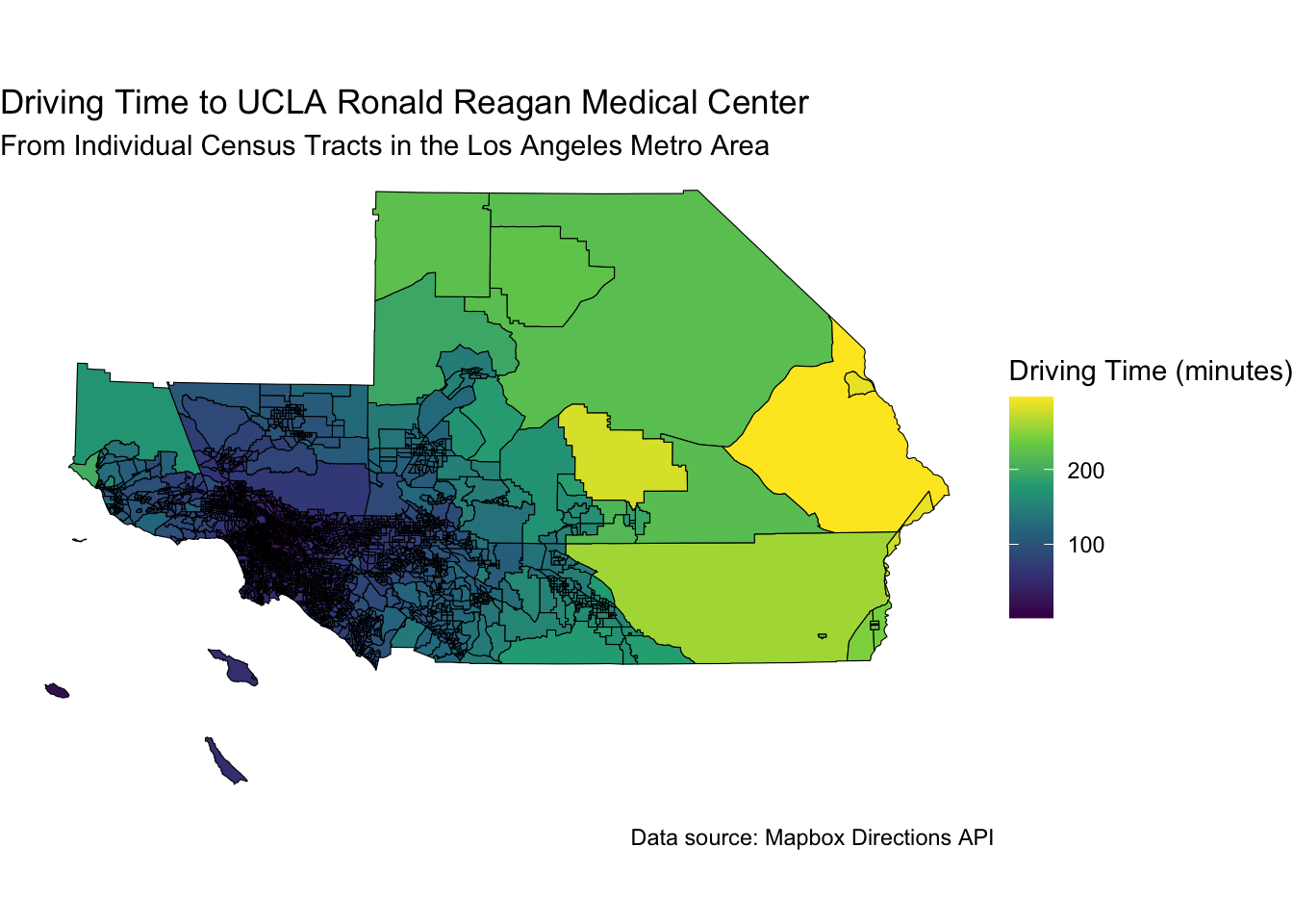
Note that for some census tracts on the east side, it can take ~ 5 hours to drive to the hospital, while for some on the west side, it can take as little as 10 minutes.
You can learn about other mapping packages, like
- general mapping ebook with chaters on tmap, ggplot2, leaflet, mapbox https://bookdown.org/nicohahn/making_maps_with_r5/docs/introduction.html
Resources for learning more about {tmap}: tmap - - Documentation at https://r-tmap.github.io/tmap/ (read the vignettes) - Book Chapter: Geocomputation with R includes a chapter on Making Maps with R, which covers tmap. - Work-in-Progress Book: Elegant and Informative Maps with tmap is an upcoming book available at tmap.geocompx.org.
Learning more about {leaflet}: Leaflet is a popular R package for creating interactive maps. - Official Leaflet for R documentation: https://rstudio.github.io/leaflet/ -
Learning more aboutusing google maps with {ggmap}: - Official ggmap documentation: https://cran.r-project.org/web/packages/ggmap/index.html - Getting started with {ggmap} https://docs.stadiamaps.com/tutorials/getting-started-in-r-with-ggmap/ - Guide - https://builtin.com/data-science/ggmap
Now let’s look :::challenge
:::