Chapter 30 Mapping Population By County
We can also use R to map population data by county. We will zoom out to the entire state of Michigan.
This will require data from the US Census Bureau, which we can get using the {tidycensus} package.
You can search for data fields at the census website at
https://data.census.gov/table/, or use the load_variables() function in the {tidycensus} package. This one is a bit fancier, as it links a county map
with an interactive plot of income by county, using the {ggiraph} package.
Run the code below, then zoom it (with the zoom button at top left of the Plots
window) to see the details. Hover over each county to see the name and its
location on the plot.
See if you can find Wayne, Washtenaw, Keewenaw, and Leelenau counties.
Which counties have the highest and lowest incomes? Which have the most income disparity (wide CI bars)?
# Load required libraries
library(tidycensus)
#library(mapboxapi)
library(mapgl)
library(sf)
library(dplyr)
library(RColorBrewer)
library(tidyverse)

# you need to set up a Census API key
# go to the Developers website https://www.census.gov/data/developers.html
# then click on the button for "Request a Key"
# you will need to create a free account
# then you can request a key
# it will be emailed to you
# Save this key in your .Renviron file as CENSUS_API_KEY

# Set your Census API key in the code
# census_api_key("YOUR_API_KEY_HERE", install = TRUE)


# Get population data by county for Michigan
michigan_population <- get_acs(
  geography = "county",
  variables = "B01003_001", # Total population variable
  state = "MI",
  year = 2022, # Most recent available year
  survey = "acs5",
  geometry = TRUE, # Include geographic boundaries
  cache_table = TRUE
)
## Getting data from the 2018-2022 5-year ACS# Clean and prepare the data
michigan_population <- michigan_population %>%
rename(population = estimate) %>%
mutate(
county_name = gsub(" County, Michigan", "", NAME),
# Create population categories for better visualization
pop_category = case_when(
population < 50000 ~ "< 50K",
population < 100000 ~ "50K - 100K",
population < 250000 ~ "100K - 250K",
population < 500000 ~ "250K - 500K",
population >= 500000 ~ "500K+"
),
pop_category = factor(pop_category,
levels = c(
"< 50K", "50K - 100K", "100K - 250K",
"250K - 500K", "500K+"
)
)
) %>%
filter(!is.na(population))
# Transform to appropriate CRS for Michigan
michigan_population <- st_transform(michigan_population, crs = 3857)
# Create choropleth map using mapbox
# plot(michigan_population["population"])
ggplot(data = michigan_population, aes(fill = population)) +
geom_sf() +
scale_fill_distiller(
palette = "RdPu",
direction = 1
) +
labs(
title = "Michigan Population by County, 2022",
caption = "Data source: 2022 1-year ACS, US Census Bureau",
fill = "ACS estimate"
) +
theme_void()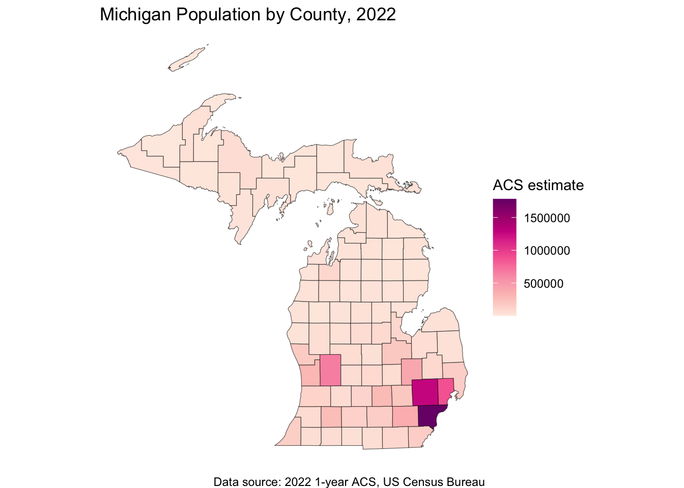
# linked maps
library(tigris)
library(tidycensus)
library(ggiraph)
library(tidyverse)
library(patchwork)
library(scales)
##
## Attaching package: 'scales'## The following object is masked from 'package:mapgl':
##
## number_format## The following object is masked from 'package:purrr':
##
## discard## The following object is masked from 'package:readr':
##
## col_factormi_income <- get_acs(
geography = "county",
variables = "B19013_001",
state = "MI",
year = 2022,
geometry = TRUE
) %>%
mutate(NAME = str_remove(NAME, " County, Michigan"))## Getting data from the 2018-2022 5-year ACSmi_map <- ggplot(mi_income, aes(fill = estimate)) +
geom_sf_interactive(aes(data_id = GEOID, tooltip = estimate)) +
scale_fill_distiller(
palette = "Blues",
direction = 1,
guide = "none"
) +
theme_void()
mi_plot <- ggplot(mi_income, aes(
x = estimate, y = reorder(NAME, estimate),
fill = estimate
)) +
geom_errorbar(aes(xmin = estimate - moe, xmax = estimate + moe)) +
geom_point_interactive(
color = "black", size = 4, shape = 21,
aes(data_id = GEOID)
) +
scale_fill_distiller(
palette = "Blues", direction = 1,
labels = label_dollar()
) +
scale_x_continuous(labels = label_dollar()) +
labs(
title = "Household income by county in Michigan",
subtitle = "2016-2020 American Community Survey",
y = "",
x = "ACS estimate (bars represent margin of error)",
fill = "ACS estimate"
) +
theme_linedraw(base_size = 8)
girafe(ggobj = mi_map + mi_plot, width_svg = 12, height_svg = 9) %>%
girafe_options(opts_hover(css = "fill:red;"))30.1 Finding a Census Field
# You can search for variables by running
vars <- load_variables(2023, "acs5", cache = TRUE)
# View(vars)library(tidycensus)
library(tidyverse)
library(crsuggest)
library(sf)
# Example: Get median household income data for tracts in a specific county with geometry
data_sf <- get_acs(
state = "MI",
county = "Washtenaw",
geography = "tract",
variables = "B19013_001", # Median household income
geometry = TRUE, # includes shapefiles
year = 2023
)## Getting data from the 2019-2023 5-year ACS## Using the projected CRS NAD83 / Michigan South which uses 'm' for measurement units. Please visit https://spatialreference.org/ref/epsg/26990/ for more information about this CRS. # Plotting the data
data_sf %>%
ggplot(aes(fill = estimate)) +
geom_sf(color = 'black') + # 'color = NA' removes the outline of the polygons
scale_fill_viridis_c(option = "viridis") + # Example color scale
labs(title = "Median Household Income by Census Tract",
subtitle = "Washtenaw County, 2023 ACS Estimates") +
coord_sf(crs = wc_crs) +
theme_void() # Removes axes and grid lines for a cleaner map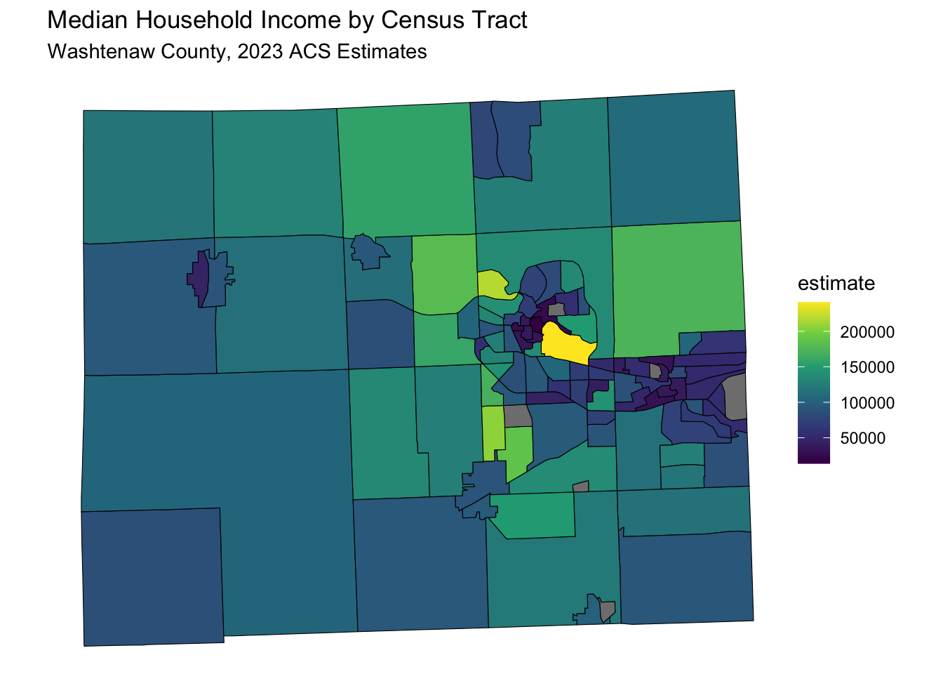
30.1.1 Mapping Commute Times
data_sf <- get_acs(
      state = "CA",
      county = "Los Angeles",
      geography = "tract",
      variables = "B08134_020", # Commute > 1 hour by car
      #"B08128_061", # Work from Home
      geometry = TRUE, # includes shapefiles
      year = 2023
    )
## Getting data from the 2019-2023 5-year ACS data_sf %>%
ggplot(aes(fill = estimate)) +
geom_sf(color = 'black') + # 'color = NA' removes the outline of the polygons
scale_fill_viridis_c(option = "viridis") + # Example color scale
labs(title = "Number Who Commute > 1 hour by Car by Census Tract",
subtitle = "Los Angeles County, 2023 ACS Estimates") +
coord_sf(crs = wc_crs) +
theme_void() # Removes axes and grid lines for a cleaner map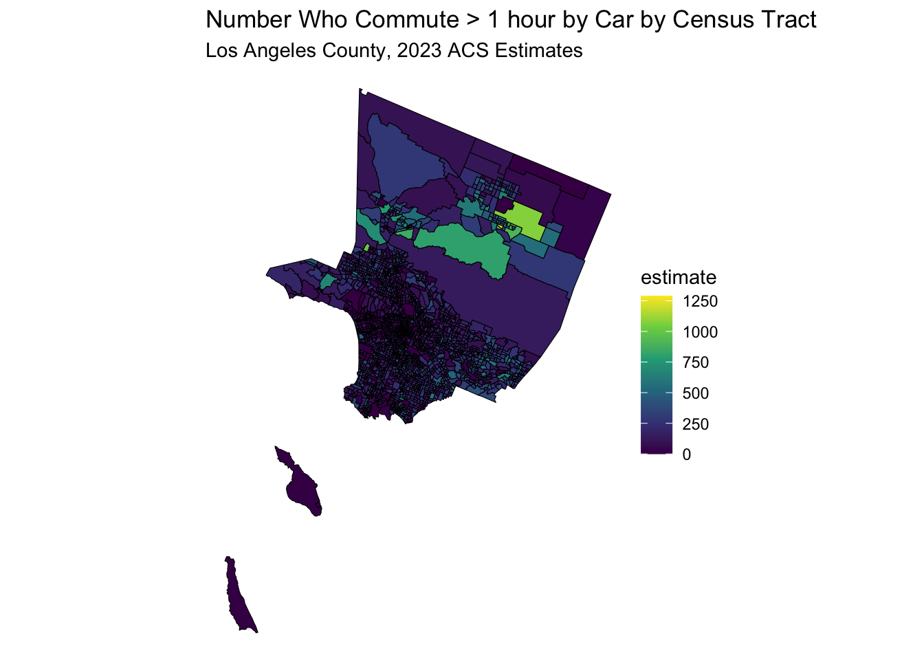
data_sf <- get_acs(
      state = "CT",
      county = "Fairfield",
      geography = "tract",
      variables = "B08134_020", # Commute > 1 hour by car
      geometry = TRUE, # includes shapefiles
      year = 2021
    )
## Getting data from the 2017-2021 5-year ACS data_sf %>%
ggplot(aes(fill = estimate)) +
geom_sf(color = 'black') + # 'color = NA' removes the outline of the polygons
scale_fill_viridis_c(option = "viridis") + # Example color scale
labs(title = "Number Who Commute > 1 hour by Car by Census Tract",
subtitle = "Fairfield County, CT, 2023 ACS Estimates") +
coord_sf(crs = wc_crs) +
theme_void() # Removes axes and grid lines for a cleaner map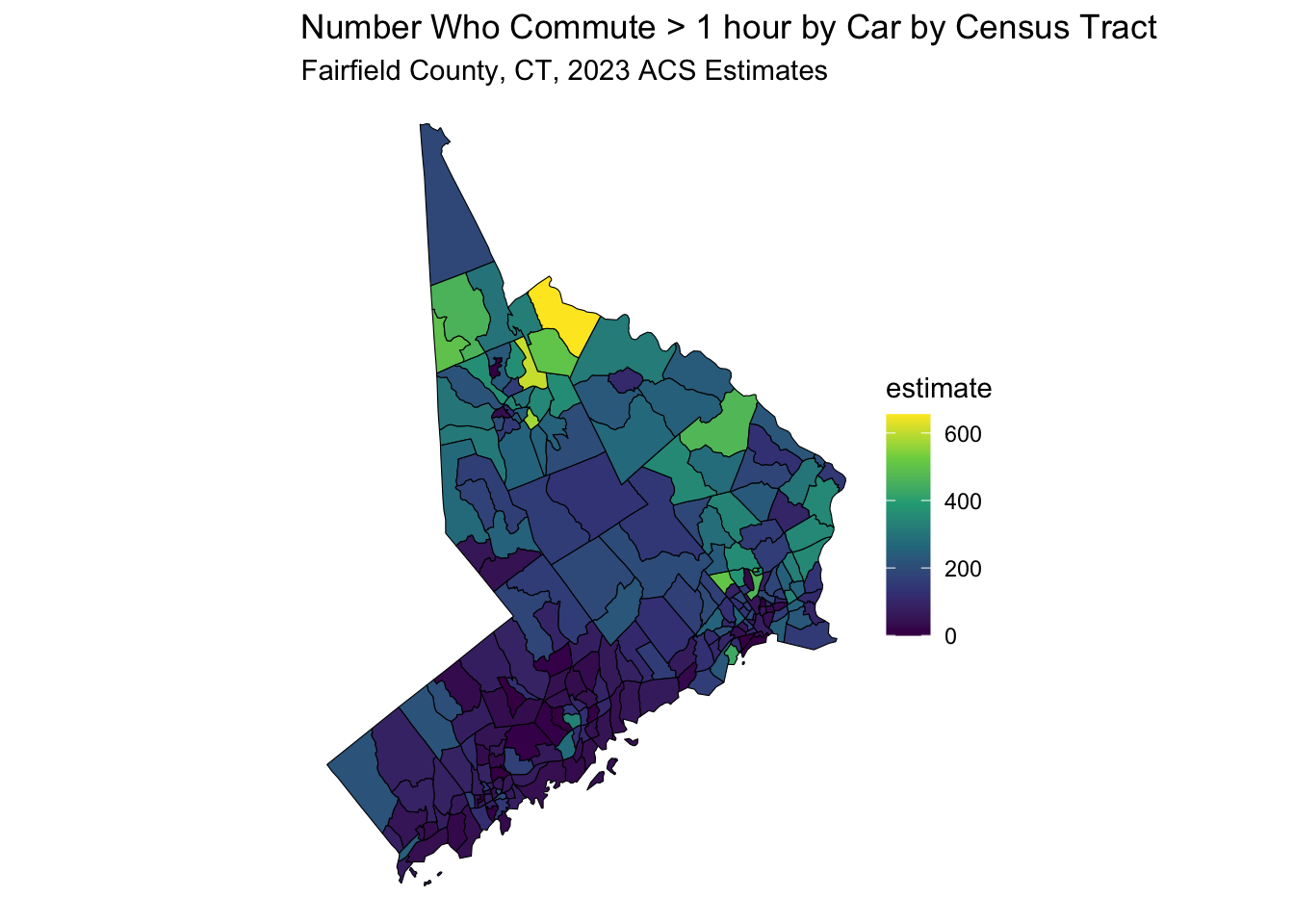
30.1.2 Mapping Work From Home
data_sf <- get_acs(
      state = "NY",
      county = "New York",
      geography = "tract",
      variables = "B08128_061", # Work from Home
      geometry = TRUE, # includes shapefiles
      year = 2023
    )
## Getting data from the 2019-2023 5-year ACS data_sf %>%
ggplot(aes(fill = estimate)) +
geom_sf(color = 'black') + # 'color = NA' removes the outline of the polygons
scale_fill_viridis_c(option = "viridis") + # Example color scale
labs(title = "Number Who Work From Home by Census Tract",
subtitle = "New York County, 2023 ACS Estimates") +
coord_sf(crs = wc_crs) +
theme_void() # Removes axes and grid lines for a cleaner map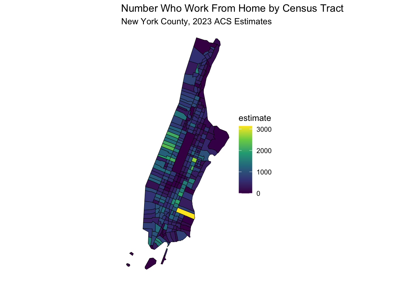
30.2 Mapping and Merging Health Data
Lets start by downloading a data set by county, from the North Carolina Institute of Medicine (NCIOM), which has a downloadable Excel spreadsheet
with health data by county. This can be found at:
https://nciom.org/nc-health-data/map/
Look for the Download Data button at the lower left.
Click on this button to download and save the Excel file to your computer,
for now, in your Downloads folder.
We will go step by step on how to will this data into R, and merge it with Census data for counties in North Carolina.
Set up a folder to be the directory for this project,
and name it something like nc_health.
Create a folder named ‘data’ within this folder.
Then save the datafile as nciom_health_data.xlsx in the data directory.
Then make the nc_health folder into a New R project.
Then, in this folder, create a new quarto file called nc_health_data.qmd.
Then copy the code below into a code chunk in the quarto file, and run the code below to read in the data.
## here() starts at /Users/peterhiggins/Documents/RCode/rmrwr-booknciom_health_data <- read_excel(here("data/nciom_health_data.xlsx"),
col_names = TRUE, skip = 1) |>
janitor::clean_names() ## New names:
## • `` -> `...1`
## • `` -> `...2`
## • `` -> `...3`
## • `` -> `...4`
## • `` -> `...5`
## • `` -> `...6`
## • `` -> `...7`Now, take a look at this data. It has variables in the leftmost column, and the counties as columns. This is a bit problematic for merging with shapefile data, which is usually in a long format, with one row per county. We will need to pivot this data to a long format, with one row per county and one column per variable.
nciom_health_data_long <- nciom_health_data |>
  select(x2, x3, alamance:yancey) |>
  pivot_longer(cols = !x2:x3, names_to = "county",
               values_to = "value") |>
  mutate(county = str_replace_all(county, "_", ""))
Now this is in long format by county in lower case, with variables names and definitions in the first two columns. We can now merge this with the Census data for North Carolina counties (as long as we make the county names clean and in lower case)
nc_population <- get_acs(
  geography = "county",
  variables = "B01003_001", # Total population variable
  state = "NC",
  year = 2021,
  survey = "acs5",
  geometry = TRUE, # Include geographic boundaries
  cache_table = TRUE
)
## Getting data from the 2017-2021 5-year ACSNote that all the county names have a single word, followed by “County, North Carolina”. How will we remove this bit and make the county names lower case? Google “R remove text from string” and you will find the str_extract function, which is part of the stringr package, which is part of the tidyverse. Try to mutate the county name to a clean lower case name
30.2.1 Solution
nc_population <- nc_population %>%
  mutate(county = str_extract(NAME, ".+(?= County, North Carolina)")) %>%
  mutate(county = tolower(county)) %>%
  mutate(county = str_replace_all(county, " ", "")) %>% # Remove spaces) |>
  mutate(county = str_trim(county)) %>% # Trim whitespace
  select (GEOID, county, geometry)
30.3 Now to merge
We want to add the geometry from the nc_population data to the nciom_health_data_long data, in a one to many merge. Let’s start with the nciom_health_data_long data (the one), and then merge it with the nc_population data (the many).
nc_merged <- nciom_health_data_long %>%
  left_join(nc_population, by = "county") %>%
  rename(variable = x2, definition = x3) %>%
  mutate(value = as.numeric(value)) # Ensure value is numeric
## Warning: There was 1 warning in `mutate()`.
## ℹ In argument: `value = as.numeric(value)`.
## Caused by warning:
## ! NAs introduced by coercionnc_merged %>%
filter(variable == "Opioid Prescribing Rate") |>
ggplot(aes(fill = value)) +
geom_sf(aes(geometry = geometry), color = 'black') +
scale_fill_viridis_c(option = "viridis") + # Example color scale
labs(title = "Opioid Prescribing Rate by County",
subtitle = "North Carolina, 2021 NCIOM Estimates") +
theme_void() # Removes axes and grid lines for a cleaner map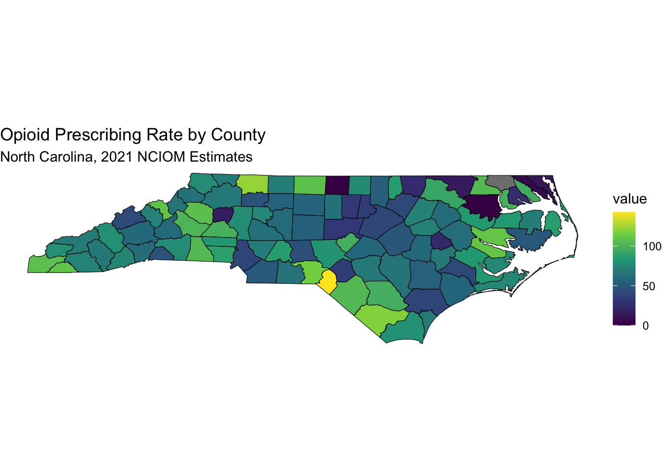
Note that Scotland County has 142.7 opioid prescriptions per 100 people, while Wake County has 41.1.
30.4 Texas Health Data
Now let’s download some health data for Texas, from the Texas Health Data website. Go to:
https://www.countyhealthrankings.org/health-data/texas/data-and-resources
Dowlnoad the first linked file, named 2025 Texas Health Data,
and save it in the data folder of your project, as texas_health_data.xlsx.
Then copy the code below into a code chunk in your quarto file, and run it to read in the data.
texas_health_data <- read_excel(here("data/texas_health_data.xlsx"),
                                col_names = TRUE, skip = 1,
                                sheet =2) |>
                                  janitor::clean_names()
## New names:
## • `Unreliable` -> `Unreliable...4`
## • `95% CI - Low` -> `95% CI - Low...7`
## • `95% CI - High` -> `95% CI - High...8`
## • `National Z-Score` -> `National Z-Score...9`
## • `95% CI - Low` -> `95% CI - Low...39`
## • `95% CI - High` -> `95% CI - High...40`
## • `National Z-Score` -> `National Z-Score...41`
## • `Unreliable` -> `Unreliable...42`
## • `95% CI - Low` -> `95% CI - Low...44`
## • `95% CI - High` -> `95% CI - High...45`
## • `National Z-Score` -> `National Z-Score...46`
## • `95% CI - Low` -> `95% CI - Low...69`
## • `95% CI - High` -> `95% CI - High...70`
## • `National Z-Score` -> `National Z-Score...71`
## • `95% CI - Low` -> `95% CI - Low...73`
## • `95% CI - High` -> `95% CI - High...74`
## • `National Z-Score` -> `National Z-Score...75`
## • `National Z-Score` -> `National Z-Score...77`
## • `National Z-Score` -> `National Z-Score...84`
## • `National Z-Score` -> `National Z-Score...86`
## • `National Z-Score` -> `National Z-Score...90`
## • `National Z-Score` -> `National Z-Score...94`
## • `National Z-Score` -> `National Z-Score...98`
## • `National Z-Score` -> `National Z-Score...100`
## • `National Z-Score` -> `National Z-Score...107`
## • `95% CI - Low` -> `95% CI - Low...115`
## • `95% CI - High` -> `95% CI - High...116`
## • `National Z-Score` -> `National Z-Score...117`
## • `95% CI - Low` -> `95% CI - Low...119`
## • `95% CI - High` -> `95% CI - High...120`
## • `National Z-Score` -> `National Z-Score...130`
## • `95% CI - Low` -> `95% CI - Low...132`
## • `95% CI - High` -> `95% CI - High...133`
## • `National Z-Score` -> `National Z-Score...134`
## • `95% CI - Low` -> `95% CI - Low...152`
## • `95% CI - High` -> `95% CI - High...153`
## • `National Z-Score` -> `National Z-Score...154`
## • `National Z-Score` -> `National Z-Score...156`
## • `National Z-Score` -> `National Z-Score...158`
## • `95% CI - Low` -> `95% CI - Low...161`
## • `95% CI - High` -> `95% CI - High...162`
## • `National Z-Score` -> `National Z-Score...163`
## • `National Z-Score` -> `National Z-Score...165`
## • `Population` -> `Population...167`
## • `95% CI - Low` -> `95% CI - Low...169`
## • `95% CI - High` -> `95% CI - High...170`
## • `National Z-Score` -> `National Z-Score...171`
## • `Population` -> `Population...173`
## • `95% CI - Low` -> `95% CI - Low...175`
## • `95% CI - High` -> `95% CI - High...176`
## • `National Z-Score` -> `National Z-Score...177`
## • `National Z-Score` -> `National Z-Score...181`
## • `National Z-Score` -> `National Z-Score...185`
## • `95% CI - Low` -> `95% CI - Low...187`
## • `95% CI - High` -> `95% CI - High...188`
## • `National Z-Score` -> `National Z-Score...189`
## • `95% CI - Low` -> `95% CI - Low...197`
## • `95% CI - High` -> `95% CI - High...198`
## • `National Z-Score` -> `National Z-Score...199`
## • `National Z-Score` -> `National Z-Score...223`
## • `National Z-Score` -> `National Z-Score...225`See if you can pull the texas acs county data for population from the ACS to get the shapefiles, using the North Carolina example above, with the get_acs() function.
Then, merge the texas_health_data with the texas_population data, using the county name as the key.
30.4.1 Solution to ACS
texas_population <- get_acs(
  geography = "county",
  variables = "B01003_001", # Total population variable
  state = "TX",
  year = 2023,
  survey = "acs5",
  geometry = TRUE, # Include geographic boundaries
  cache_table = TRUE
) |>
  mutate(county = str_remove(NAME, " County, Texas")) %>%
  select (GEOID, county, geometry)
## Getting data from the 2019-2023 5-year ACS30.4.2 Solution to Merge
See if you can map the “percent_vaccinated” (for influenza) variable by county, using the same method as above.
30.4.3 Solution to Mapping
texas_merged %>%
  select(GEOID, county, percent_vaccinated, geometry) |>
    ggplot(aes(fill = percent_vaccinated)) +
    geom_sf(aes(geometry = geometry), color = NA) + #try without borders
    scale_fill_viridis_c(option = "viridis",
            name = "% Vax \nfor Flu") +
    labs(title = "Percent Vaccinated for Influenza by County",
          subtitle = "Texas, 2025 Health Data Estimates") +
    theme_void() # Removes axes and grid lines for a cleaner map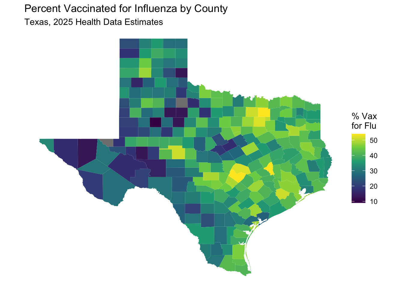
30.5 Mapping California
Let’s try mapping some health data for California, using the California Health Data website.
Go to: https://www.countyhealthrankings.org/health-data/california/data-and-resources
Download the first linked file, named 2025 California Health Data,
and save it in the data folder of your project, as california_health_data.xlsx.
Then copy the code below into a code chunk in your quarto file, and run it to read in the data.
california_health_data <- read_excel(here("data/california_health_data.xlsx"),
                                col_names = TRUE, skip = 1,
                                sheet =2) |>
                                  janitor::clean_names()
## New names:
## • `Unreliable` -> `Unreliable...4`
## • `95% CI - Low` -> `95% CI - Low...7`
## • `95% CI - High` -> `95% CI - High...8`
## • `National Z-Score` -> `National Z-Score...9`
## • `95% CI - Low` -> `95% CI - Low...39`
## • `95% CI - High` -> `95% CI - High...40`
## • `National Z-Score` -> `National Z-Score...41`
## • `Unreliable` -> `Unreliable...42`
## • `95% CI - Low` -> `95% CI - Low...44`
## • `95% CI - High` -> `95% CI - High...45`
## • `National Z-Score` -> `National Z-Score...46`
## • `95% CI - Low` -> `95% CI - Low...69`
## • `95% CI - High` -> `95% CI - High...70`
## • `National Z-Score` -> `National Z-Score...71`
## • `95% CI - Low` -> `95% CI - Low...73`
## • `95% CI - High` -> `95% CI - High...74`
## • `National Z-Score` -> `National Z-Score...75`
## • `National Z-Score` -> `National Z-Score...77`
## • `National Z-Score` -> `National Z-Score...84`
## • `National Z-Score` -> `National Z-Score...86`
## • `National Z-Score` -> `National Z-Score...90`
## • `National Z-Score` -> `National Z-Score...94`
## • `National Z-Score` -> `National Z-Score...98`
## • `National Z-Score` -> `National Z-Score...100`
## • `National Z-Score` -> `National Z-Score...107`
## • `95% CI - Low` -> `95% CI - Low...115`
## • `95% CI - High` -> `95% CI - High...116`
## • `National Z-Score` -> `National Z-Score...117`
## • `95% CI - Low` -> `95% CI - Low...119`
## • `95% CI - High` -> `95% CI - High...120`
## • `National Z-Score` -> `National Z-Score...130`
## • `95% CI - Low` -> `95% CI - Low...132`
## • `95% CI - High` -> `95% CI - High...133`
## • `National Z-Score` -> `National Z-Score...134`
## • `95% CI - Low` -> `95% CI - Low...152`
## • `95% CI - High` -> `95% CI - High...153`
## • `National Z-Score` -> `National Z-Score...154`
## • `National Z-Score` -> `National Z-Score...156`
## • `National Z-Score` -> `National Z-Score...158`
## • `95% CI - Low` -> `95% CI - Low...161`
## • `95% CI - High` -> `95% CI - High...162`
## • `National Z-Score` -> `National Z-Score...163`
## • `National Z-Score` -> `National Z-Score...165`
## • `Population` -> `Population...167`
## • `95% CI - Low` -> `95% CI - Low...169`
## • `95% CI - High` -> `95% CI - High...170`
## • `National Z-Score` -> `National Z-Score...171`
## • `Population` -> `Population...173`
## • `95% CI - Low` -> `95% CI - Low...175`
## • `95% CI - High` -> `95% CI - High...176`
## • `National Z-Score` -> `National Z-Score...177`
## • `National Z-Score` -> `National Z-Score...181`
## • `National Z-Score` -> `National Z-Score...185`
## • `95% CI - Low` -> `95% CI - Low...187`
## • `95% CI - High` -> `95% CI - High...188`
## • `National Z-Score` -> `National Z-Score...189`
## • `95% CI - Low` -> `95% CI - Low...197`
## • `95% CI - High` -> `95% CI - High...198`
## • `National Z-Score` -> `National Z-Score...199`
## • `National Z-Score` -> `National Z-Score...223`
## • `National Z-Score` -> `National Z-Score...225`Now pull the California shapefiles, using the population variable code from tidycensus. Modify the County names as needed. Then, merge the california_health_data with the california_population data, using the county name as the key.
california_population <- get_acs(
  geography = "county",
  variables = "B01003_001", # Total population variable
  state = "CA",
  year = 2023,
  survey = "acs5",
  geometry = TRUE, # Include geographic boundaries
  cache_table = TRUE
) |>
  mutate(county = str_remove(NAME, " County, California")) %>%
  select (GEOID, county, geometry)
## Getting data from the 2019-2023 5-year ACSNow merge the data, and map the “low_birth_weight” variable by county, using the same method as above.
Now map
california_merged %>%
  select(GEOID, county, percent_low_birth_weight, geometry) |>
    ggplot(aes(fill = percent_low_birth_weight)) +
    geom_sf(aes(geometry = geometry), color = NA) + #try without borders
    scale_fill_viridis_c(option = "viridis",
            name = "% Low \nBirth Weight") +
    labs(title = "Percent Low Birth Weight by County",
          subtitle = "California, 2025 Health Data Estimates") +
    theme_void() # Removes axes and grid lines for a cleaner map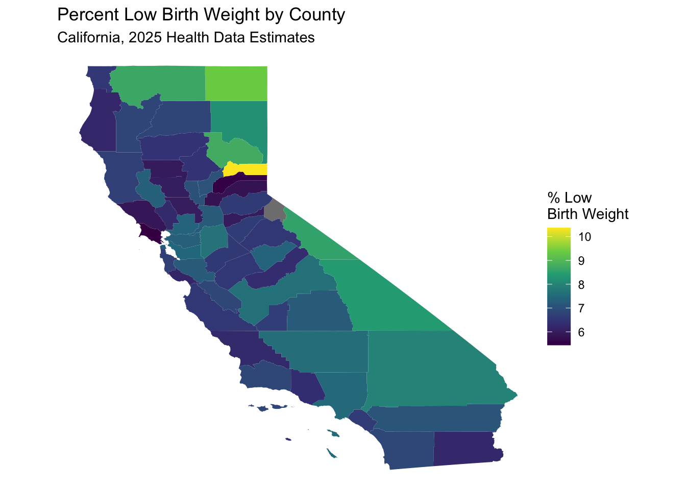
30.6 A bit of US geographic unit history
GEOID and FIPS are both geographic identifiers used by the Census Bureau to classify and organize geographic areas. FIPS (Federal Information Processing Standards) codes are a part of the GEOID structure, but GEOID encompasses a broader range of geographic levels and combinations. Essentially, a GEOID is a unique numeric code that identifies a specific geographic area, and often incorporates FIPS codes for certain levels like state and county.
FIPS Codes: . These are a set of standards developed by the National Institute of Standards and Technology (NIST). They are used to identify geographic entities like states, counties, and places. FIPS codes are often embedded within GEOIDs. FiPS codes were originally created in the 1970s and have been used in various federal datasets, including those from the Census Bureau, until 2008, when they were (largely) replaced by GEOIDs.
GEOIDs: . GEOIDs are unique, numeric identifiers assigned by the Census Bureau to various geographic areas, such as census tracts, block groups, and blocks. They are used to link census data to geographic boundaries. A GEOID is often a combination of FIPS codes and other Census Bureau codes, depending on the geographic level. For example, a census tract GEOID might include the state (2 digit) and county (3 digit) FIPS codes, along with a census tract code. In simpler terms, you can think of it like this: FIPS codes are like building blocks, and GEOIDs are like the structures built using those blocks, along with other components.
FIPS codes are an older part of the larger GEOID system. GEOIDs are used by the Census Bureau to uniquely identify and organize geographic areas for data tabulation down to the census block. FIPS codes are still used in various contexts, particularly in older datasets and systems. The Census Bureau assigns GEOIDs to a wide range of geographic entities, including those not specifically covered by FIPS codes. A longer GEOID with more digits means that it has more granularity, with extra digits representing more specific geographic areas, such as census tracts or block groups. A census tract GEOID (e.g., 53065950101) includes the state code (53), the county code (065), and the tract code (950101).
By now you may have noticed that the County Health Rankings website has
national health data in a spreadsheet as well.
If you go to:
https://www.countyhealthrankings.org/health-data/methodology-and-sources/data-documentation
You can find and download to your data folder a file named
2025 County Health Rankings National Data as something like
national_health_data.xlsx.
and you can also find a useful data dictionary file named
2025 County Health Rankings Data Dictionary.
There are also trend files available to explore.
Let’s start by examining the national data file by county.
First we will load the shapefiles and population by county for the
entire us using the get_acs function from tidycensus.