Chapter 10 Mutating Joins to Combine Data Sources
10.1 What are Joins?
Joins (sometimes called merge operations) are used to join together different datasets. This can be really helpful for joining together data from different data sources, like different forms in REDCap (demographics, vitals, visit 1 data), or the results of a data query from your electronic medical record, or national or state-level data available from sources like the CDC or a state health department. By linking these data you can find new connections, and gain a new understanding of disease, social determinants of health, or geographic factors.
10.2 What are Mutating Joins?
These are joins between a base dataset (x) and a new dataset (y) that add new variables to the base dataset, like a mutate() function in dplyr. Typically you would start with a dataset that includes one row for each observation, and often one row for each participant.
There are four types of mutating joins:
left join - all variables from the base dataset (x) are retained, and new variables from new dataset (y) that match the observations (rows) in dataset x on the key (unique id) variable are added.
right join - all variables from the new dataset (y) are retained, and new variables from the base dataset (x) that match the observations (rows) in dataset y on the key (unique id) variable are added.
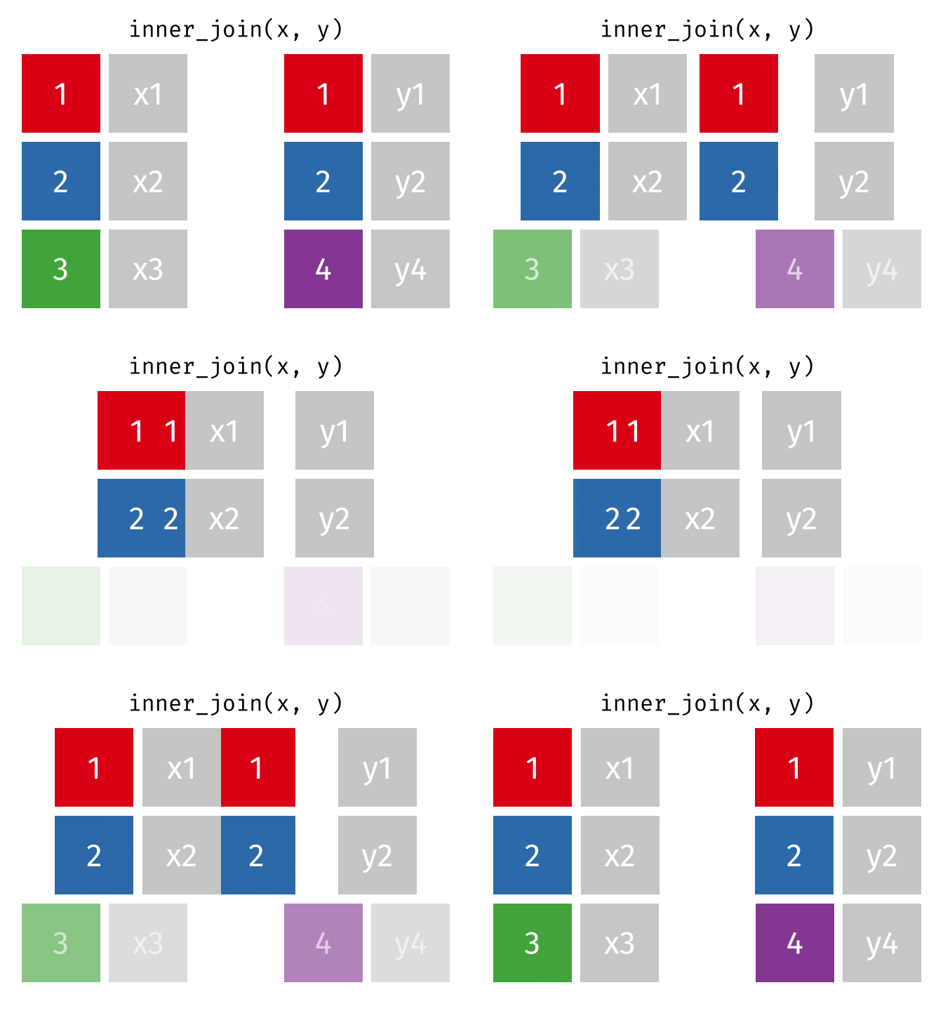
inner join - includes all rows in both dataset (x) and dataset (y), requiring matching on the key (unique id) variable.
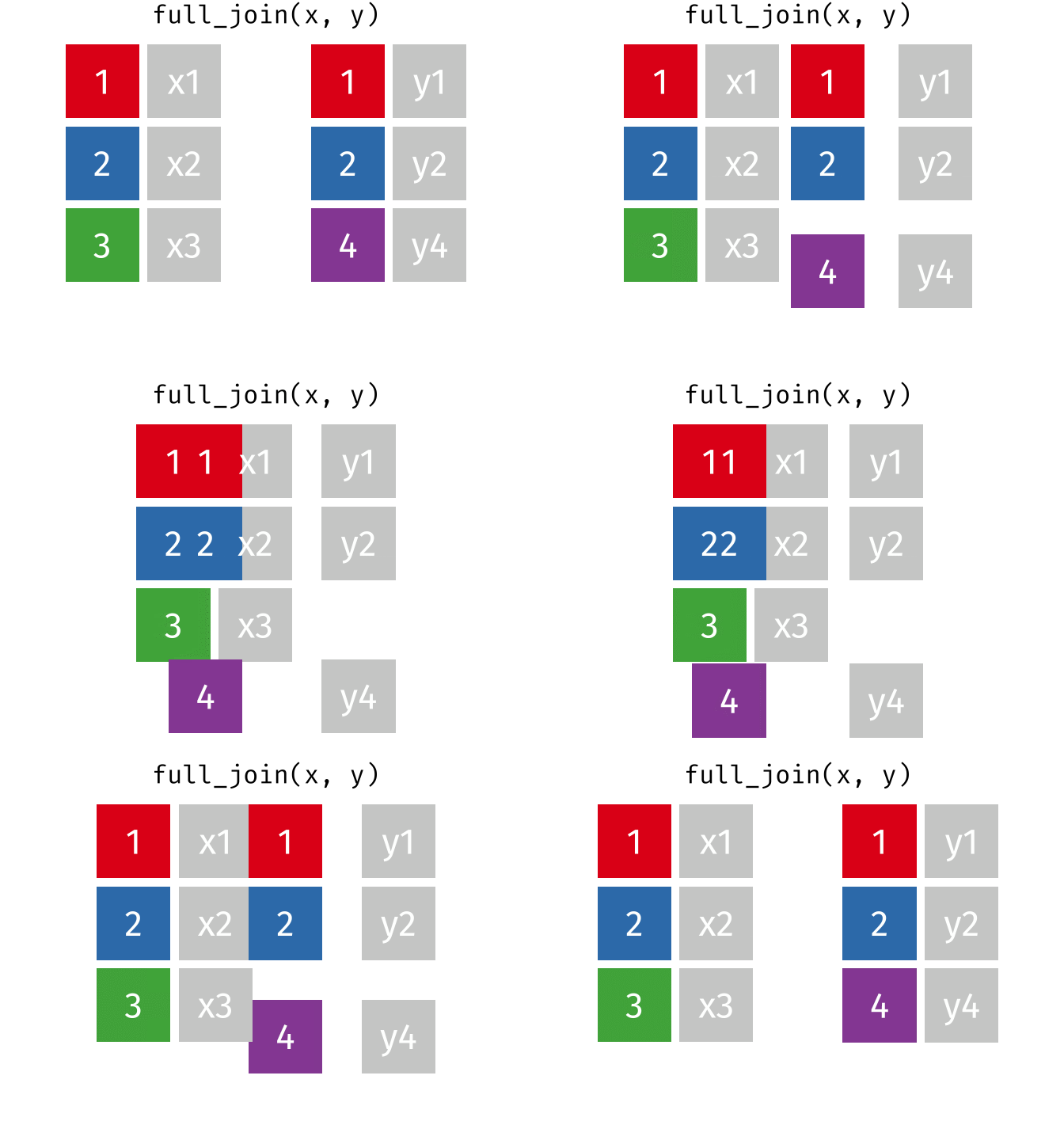
full join - includes all rows in either dataset (x) or dataset (y), matching on the key (unique id) variable when matches are present, and filling in NAs in missing columns if no match is present.
10.3 Let’s Start with Left Joins
To get started, let’s download two toy datasets - Copy and run the code chunk below to assign these to birthdays and hometowns.
birthdays <- read.csv("https://raw.githubusercontent.com/higgi13425/medicaldata/master/data-raw/join_data/birthdays.csv") %>% select(-X)

hometowns <- read.csv("https://raw.githubusercontent.com/higgi13425/medicaldata/master/data-raw/join_data/hometowns.csv") %>% select(-X)
The left join is the most common mutating join, as it allows you to start with a base dataset and add matching variables from other sources.
- left join - all variables from the base dataset (x) are retained, and new variables from new dataset (y) that match the observations (rows) in dataset x on the key (unique id) variable are added.
Let’s start with a simple left join with these two small and simple “toy” datasets about famous physicians. Start by copying and running a glimpse() function on each dataset from the code chunk below.
## Rows: 3
## Columns: 2
## $ name <chr> "Rudolf Virchow", "Virginia Apgar", "William Osler"
## $ dob <chr> "10/13/1821", "6/7/1909", "7/12/1849"## Rows: 3
## Columns: 2
## $ name <chr> "Rudolf Virchow", "Virginia Apgar", "Hippocrates"
## $ hometown <chr> "Berlin", "Westfield, NJ", "Kos"We now have two small datasets, with 3 rows each and 2 variables each. Across the toy datasets, data are provided on 4 famous physicians, so that each dataset is missing one physician from the other dataset.
The 3 main arguments of the left_join() function include
x (base dataset, or left dataset)
y (new dataset, or right dataset)
by (variable to match, known as the key, or unique id - must be unique to each observation). The dplyr functions are often smart enough to figure the keyid variable out on their own.
10.4 Left Join in Action
The animation below illustrates how a left_join works. The colored numbers represent the unique key variable, and the gray boxes represent the unique values from datasets x and y. Notice that observation 4 in dataset y, because it does not have a match in dataset x, does not end up in the final dataset.

tidyexplain
repo10.5 Left Join in Practice
Let’s see how it works. Run the code chunk below. The hometowns dataset
is x, or the base/left dataset, and the birthdays dataset is the y,
or new/right dataset. Notice that we don’t specify a variable for by.
## Joining with `by = join_by(name)`## name hometown dob
## 1 Rudolf Virchow Berlin 10/13/1821
## 2 Virginia Apgar Westfield, NJ 6/7/1909
## 3 Hippocrates Kos <NA>This produces a new dataset with 3 columns - name, hometown, and date of
birth. The left_join function figures out which is the key id variable
to match datasets on its own. You could assign this dataset to a new
object, and add more data from a 3rd, or even a 4th dataset, as long as
each has a matching unique key variable.
10.6 Quick Quiz
Which variable in the left_join above is the key unique variable present in both datasets that is used to join these two datasets?
Why does Hippocrates have an NA for date of birth?
This is great - left_join() figured out how to match up the observations on its own. But sometimes it is not obvious how to match up observations.
To play it safe, you should specify the matching unique key id variable.
In this case, the common variable to the two datasets is “name”. You
specify this with the by variable in quotes, as in the below code
chunk
##             name      hometown        dob
## 1 Rudolf Virchow        Berlin 10/13/1821
## 2 Virginia Apgar Westfield, NJ   6/7/1909
## 3    Hippocrates           Kos       <NA>
This gets complicated when the intended matching variable does not quite match.
A common “gotcha” when joining datasets is not having an exact match of the intended by variable.
Common scenarios include:
- mismatched spelling or capitalization of the variable name
- mismatch in the variable data type: integers and numbers look the same, but if they are not the same data type, the join will fail.
It is important to:
- glimpse() both datasets, and check the name of the intended by variable in both datasets.
- glimpse() both datasets, and check the data type of the intended by variable in both datasets.
- predict the number of rows and columns in the resulting dataset after the join - if it is way off, something is wrong (a really important reality check)
10.7 Problem variable names
Sometimes your variable names will be just a bit off. Read in this new version of hometowns2 by copying and running the code below.
hometowns2 <- read.csv("https://raw.githubusercontent.com/higgi13425/medicaldata/master/data-raw/join_data/hometowns2.csv") %>% select(-X)Now write your own left join of hometowns2 and birthdays using the code below as a starting point. Remember to glimpse( ) the new dataset first.
## Error in `left_join()`:
## ! Join columns in `x` must be present in the data.
## ✖ Problem with `name`.
10.8 Right Join in Action
The animation below illustrates how a right_join works. The colored numbers represent the unique key variable, and the gray boxes represent the unique values from datasets x and y. Notice that observation 3 in dataset x, because it does not have a match in dataset y, does not end up in the final dataset. In a right join, the y dataset is considered the base dataset, and the matching observations from the x dataset are added. This is not very different from a left_join, but occurs in a different order.

tidyexplain
repo10.9 Right Join in Practice
Let’s see how it works. Run the code chunk below. The hometowns dataset
is x, or the base/left dataset, and the birthdays dataset is the y,
or new/right dataset. Notice that we don’t specify a variable for by.
## Joining with `by = join_by(name)`## name hometown dob
## 1 Rudolf Virchow Berlin 10/13/1821
## 2 Virginia Apgar Westfield, NJ 6/7/1909
## 3 William Osler <NA> 7/12/1849This produces a new dataset with 3 columns - name, hometown, and date of
birth. Notice that this result id different from the left_join
result above. William Osler appears (without a hometown, as he was born
in the wilds of Ontario), and Hippocrates does not. Which dataset is the
base dataset affects the result of the join.
The right_join function figures out which is the key id variable to
match datasets on its own. You could assign this dataset to a new
object, and add more data from a 3rd, or even a 4th dataset, as long as
each has a matching unique key variable.
Most people entirely use left_join(), rather than right_join(), for the sake of consistency. The main time you might want to use a right_join()() is when you have a base dataset, and you want to add some variables from a new dataset, but the new dataset needs some wrangling and selecting variables first. In this case, you can do your wrangling of the new dataset, then right_join() it to your base dataset. This will add the new variables to the base dataset.
A simple example is shown below. We want to add the dataset hometowns2 to the dataset birthdays, but we first have to remove an extra variable (X), and fix the “Name” variable name. Then we can pipe the resulting dataset into the join. But if we pipe it into a left_join(), hometowns will by default become the base (x) dataset, as it comes first. If we want to keep birthdays as the base (x) dataset, we can use a right_join(). This will result in a table in which everyone has a known birthday, but not necessarily a known hometown.
hometowns2 <- read.csv("https://raw.githubusercontent.com/higgi13425/medicaldata/master/data-raw/join_data/hometowns2.csv") %>%
  select(-X) %>%
  purrr::set_names(c("name", "hometown"))
hometowns2 %>%
  right_join(birthdays)
## Joining with `by = join_by(name)`## name hometown dob
## 1 Rudolf Virchow Berlin 10/13/1821
## 2 Virginia Apgar Westfield, NJ 6/7/1909
## 3 William Osler <NA> 7/12/184910.10 Inner Joins
The inner join only keeps observations for which there is a matching observation in both datasets. Think of the inner_join as the intersection of the two sets. Here is an animation of what this looks like

tidyexplain
repoFor birthdays and hometowns, what do you predict the result will be? Look at the datasets below (run the glimpse code) and take a guess.
## Rows: 3
## Columns: 2
## $ name <chr> "Rudolf Virchow", "Virginia Apgar", "William Osler"
## $ dob <chr> "10/13/1821", "6/7/1909", "7/12/1849"## Rows: 3
## Columns: 2
## $ name <chr> "Rudolf Virchow", "Virginia Apgar", "Hippocrates"
## $ hometown <chr> "Berlin", "Westfield, NJ", "Kos"10.11 Quick Quiz
How many rows will result if you inner_join birthdays with hometowns?
Which physicians will appear in this resulting table?
10.13 Full Joins
The full (aka outer) join keeps all observations for from both datasets, whether or not there is a match. Think of the full_join as the union of the two sets. Here is an animation of what this looks like

tidyexplain
repoFor birthdays and hometowns, what do you predict the result will be? Look at the datasets below (run the glimpse code) and take a guess.
## Rows: 3
## Columns: 2
## $ name <chr> "Rudolf Virchow", "Virginia Apgar", "William Osler"
## $ dob <chr> "10/13/1821", "6/7/1909", "7/12/1849"## Rows: 3
## Columns: 2
## $ name <chr> "Rudolf Virchow", "Virginia Apgar", "Hippocrates"
## $ hometown <chr> "Berlin", "Westfield, NJ", "Kos"10.14 Quick Quiz
How many rows will result if you full_join birthdays with hometowns?
Which physicians will appear in this resulting table?
10.15 Now Let’s take a Look at the result
## Joining with `by = join_by(name)`## name dob hometown
## 1 Rudolf Virchow 10/13/1821 Berlin
## 2 Virginia Apgar 6/7/1909 Westfield, NJ
## 3 William Osler 7/12/1849 <NA>
## 4 Hippocrates <NA> KosThe full_join does not require matches, so all observations from both datasets, appear in the full_join result.