Chapter 5 Importing Your Data into R
For most of this book, we will be using datasets from the {medicaldata} package.
These are easy to load.
If you type into the Console pane medicaldata::scurvy , you will get James Lind’s scurvy dataset (actually, a reconstruction of what it might have looked like for his 12 participants).
If you want to save this data to an object in your work environment, you just need to assign this to a named object, like scurvy, like so, with an assignment arrow, composed of a less than sign (<) and a hyphen (-):
scurvy <- medicaldata::scurvy

# now print the columns for id and treatment
scurvy %>%
  select(study_id:treatment) |>  #this selects columns
  slice_tail(n = 7) #slices last seven rows
## # A tibble: 7 × 2
## study_id treatment
## <chr> <fct>
## 1 006 vinegar
## 2 007 sea_water
## 3 008 sea_water
## 4 009 citrus
## 5 010 citrus
## 6 011 purgative_mixture
## 7 012 purgative_mixtureThere are a number of medical datasets to explore and learn with, within the {medicaldata} package.
However, at some point, you will want to use R to work on your own data. You may already be itching to get started on your own data. This is a good thing. Working with your own data, toward your own goals, will be a motivating example, and will help you learn R. As you go through the different chapters, use the example data and exercises to get you started and to learn the principles, and then try what you have learned on your own data.
Reproducibility and Raw Data
It is an important principle to always save an untouched copy of your raw data.
You can copy it to a new object, and experiment with modifying it, cleaning it, making plots, etc., but always leave the original data file untouched.
You want to create a completely reproducible, step-by-step, scripted trail from your raw data to your finished analysis and final report, and you can only do that if you preserve the original raw data.
That is the cornerstone of your analysis.
It is tempting to fix minor data entry errors, or other aspects of the raw data.
Do not do this - leave all errors intact in your raw data, and explicitly make edits with explanations of
- who made the edit
- when it was made
- what was changed
- and why the edit was made.
You should provide a justification for each change, and identify source documents to support the rationale. Every edit should be documented in your code, with who, when, what, and why.
Now, on to the fun part. Let’s read in some data!
5.1 Reading data with the {readr} package
Many of the standard data formats can be read with functions in the {readr} package. This package is part of the {tidyverse} meta-package. These functions include:
- read_csv() for comma-separated values (*.csv) files
- read_tsv() for tab-separated values (*.tsv) files
- read_delim() for files with a different delimiter that you can specify (instead of commas or tabs, there might be semicolons), or you can let {readr} guess the delimiter in readr 2.0.
- read_fwf() for fixed width files
- read_table() for tabular files where columns are separated by white-space.
- read_log() is specifically for web log files
Let’s read a csv file.
First, make sure that you have the {readr} package loaded (or the {tidyverse} meta-package, which includes {readr}).
You can load {readr} with the library() function, if you have already installed this package.
library(readr)
# or you can use
library(tidyverse) # which will load 8 packages, including readr
# the other 7 packages are ggplot, tibble, tidyr, dplyr, purrr, stringr, and forcats
Note that this will not work if you do not already have the {readr} package installed on your computer.
You will get an error, like this: Error in library(readr) : there is no package called 'readr'
This is not a big problem - but you have to install the package first, before you can load it.
You only need to do this once, like buying a book, and putting it in your personal library.
Each time you use the package, you have to pull the book off the shelf, with library(packagename).
To install the {readr} package, we can install the whole {tidyverse} package, which will come in handy later.
Just enter the following in your Console pane to install the {tidyverse} meta-package:
install.packages('tidyverse')
Note that quotes around ‘tidyverse’ are required, as tidyverse is not yet a known object or package in your working environment.
Once the {tidyverse} package is installed, you can use library(tidyverse) without quotes, as it is a known (installed) package.
We will also want to use the {glue} package shortly to access files on the web. Practice installing this package. Copy and run the code chunk below in your RStudio Console panel to install and load the {glue} package.
OK, after that detour, we should be all caught up - you should be able to run library(tidyverse) or library(readr) or library(glue) without an error.
Now that you have {readr} loaded, you can read in some csv data.
Let’s start with a file named scurvy.csv in a data folder on GitHub. You will need to glue together the url_stem (the first part of the path to the web address) and “data/scurvy.csv” (the folder and file name) to get the full web address. Copy and run the code chunk below to see the url_stem and the dataset.
## [1] "https://raw.githubusercontent.com/higgi13425/rmrwr-book/master/"## Rows: 12 Columns: 8
## ── Column specification ────────────────────────────────────────────────────────
## Delimiter: ","
## chr (8): study_id, treatment, dosing_regimen_for_scurvy, gum_rot_d6, skin_so...
##
## ℹ Use `spec()` to retrieve the full column specification for this data.
## ℹ Specify the column types or set `show_col_types = FALSE` to quiet this message.## # A tibble: 12 × 8
## study_id treatment dosing_regimen_for_s…¹ gum_rot_d6 skin_sores_d6
## <chr> <chr> <chr> <chr> <chr>
## 1 001 cider 1 quart per day 2_moderate 2_moderate
## 2 002 cider 1 quart per day 2_moderate 1_mild
## 3 003 dilute_sulfuric_acid 25 drops of elixir of… 1_mild 3_severe
## 4 004 dilute_sulfuric_acid 25 drops of elixir of… 2_moderate 3_severe
## 5 005 vinegar two spoonfuls, three … 3_severe 3_severe
## 6 006 vinegar two spoonfuls, three … 3_severe 3_severe
## 7 007 sea_water half pint daily 3_severe 3_severe
## 8 008 sea_water half pint daily 3_severe 3_severe
## 9 009 citrus two lemons and an ora… 1_mild 1_mild
## 10 010 citrus two lemons and an ora… 0_none 0_none
## 11 011 purgative_mixture a nutmeg-sized paste … 3_severe 3_severe
## 12 012 purgative_mixture a nutmeg-sized paste … 3_severe 3_severe
## # ℹ abbreviated name: ¹dosing_regimen_for_scurvy
## # ℹ 3 more variables: weakness_of_the_knees_d6 <chr>, lassitude_d6 <chr>,
## # fit_for_duty_d6 <chr>Let’s look at what was extracted from the csv file. This starts after the url_stem (web address) is printed out.
The Console pane has a
the number of rows (12) and columns (8) in the dataset.
The Column specification, followed by
the data in rectangular format.
In the Column specification, the delimiter between items of data is identified (a comma), and a listing of variables with the character (chr) data type is printed. There are no non-character data types in this particular dataset.
The ‘guessing’ of what data type is appropriate for each variable is done ‘automagically’, as the read_csv() function reads the first 1000 rows, then guesses what data type is present in each column (variable).
It is often conservative, and in this case, made all of these columns into character variables (also called strings).
You could argue that the col_character() assignment should be numeric for the study_id variable, or that the Likert scales used for outcomes like gum_rot_d6 and skin_sores_d6 should be coded as ordinal categorical variables, known as ordered factors in R.
You will learn to control these data types during data import with the spec() argument.
The last piece of output is the data rectangle itself.
This is first identified as a ‘tibble’, which is a type of data table, with 12 rows and 8 columns, in # A tibble: 12 x 8.
This is followed by a header row of variable names, and just below that is the data type (<chr> for character) for each column.
Then, on the left are gray row numbers (which are not actually part of the data set), followed by (to the right) rows of data.
A tibble, by default, only prints out only as many rows of data as will fill the console, and no more columns than will fill the width of your current console window.
The other columns (variable names) are listed in order at the bottom of the tibble in gray type.
Now, by simply reading in the data, you can look at it, but you can’t do anything with it, as you have not saved it as an object in your working Environment.
If you want to do things with this data, and make them last, you have to assign the data to an object, and give it a name.
To do this, you need to use an assignment arrow, as below, where the data is assigned to the object, scurvy_data.
## Rows: 12 Columns: 8
## ── Column specification ────────────────────────────────────────────────────────
## Delimiter: ","
## chr (8): study_id, treatment, dosing_regimen_for_scurvy, gum_rot_d6, skin_so...
##
## ℹ Use `spec()` to retrieve the full column specification for this data.
## ℹ Specify the column types or set `show_col_types = FALSE` to quiet this message.Now this is saved to scurvy_data in your working Environment.
You can now look in the Environment tab (top right pane in RStudio) and see that scurvy_data has now appeared in the Data section, with 12 observations of 8 variables.
This is not a file written (saved) to disk, but this dataset is now available in the working environment as an assigned data object.
You can click on the blue arrow next to scurvy_data to show the variable names and variable types for this dataset.
You can also click on the name scurvy_data to open up a Viewer window in the top left (Source) pane. You can scroll around to inspect all of the data. You can also get this view by typing View(scurvy_data) into the Console pane.
You can also print out the data to the Console pane at any time by typing scurvy_data into the Console, or into a script. Try this out in the Console pane.
5.1.1 Test yourself on scurvy
Inspect the data in the Viewer, and find each answer.
- How many limes did the British seamen in the citrus arm receive each day?
You can also start with the scurvy_data object, and do things to this data object, like summarize it, or graph it, or calculate total_symptom_score in a data pipeline.
Once you have assigned your data to an object, it will stick around in that R session for later use. Your changes will disappear when you close the session, unless you save it to disk, with functions like save() or write_csv().
The csv (comma separated values) format is a very common data format, and most data management programs have a way to export *.csv files.
The csv format is simple, is not owned by anyone, and works across platforms.
However, it can occasionally be tricky if you have commas in the middle of a variable like degree, with entries like ‘md, phd’ in a column that is mostly ‘md’.
The read_csv function is pretty smart, and usually gets the number of columns right, but this is something to watch out for.
Notice that read_csv had no problem with the dosing of vinegar (“two spoonfuls, three times a day”) in the scurvy dataset, despite multiple commas.
If you happen to come across a tab-separated values file, read_tsv() works the same way. Both of these functions have reasonable defaults, so that most of the time, you just have to use the path to your file (usually on your hard drive, rather than on the web) as the only argument. On occasion, though, you will want to take control of some of the other arguments, and use something other than the defaults.
5.1.2 What is a path?
A path is the trail through the folders in your hard drive (or on the web) that the computer needs to follow to find a particupar file. Paths can look something like:
- C:/Documents/Rcode/my_file.R
- ~/User/Documents/Rcode/my_file.R
and can get pretty complicated to keep track of. One particularly nice feature of Projects in RStudio is that the project directory is always your home, or root directory. You can make your life easier by using the {here} package, which memorizes the path to your project, so you can just write here(my_file.R), and not have to worry about making a typo in a long path name.
When your data has no column names (headers), read_csv will (by default) assume that the first row of the data is the column names.
To fix this, add the argument, col_names = FALSE.
You can also assign your own col_names by setting a vector, like c(“patient_id”, “treatment”, “outcome”) [note that c() concatenates data items into a vector] equal to to col_names, as below. Copy and run this code chunk in your RStudio Console pane to see how the output is different.
read_csv(file = glue(url_stem, 'data/scurvy.csv'),
col_names = c("pat_id", "arm", "dose", "gums", "skin", "weak", "lass", "fit"))
## Rows: 13 Columns: 8
## ── Column specification ────────────────────────────────────────────────────────
## Delimiter: ","
## chr (8): pat_id, arm, dose, gums, skin, weak, lass, fit
##
## ℹ Use `spec()` to retrieve the full column specification for this data.
## ℹ Specify the column types or set `show_col_types = FALSE` to quiet this message.## # A tibble: 13 × 8
## pat_id arm dose gums skin weak lass fit
## <chr> <chr> <chr> <chr> <chr> <chr> <chr> <chr>
## 1 study_id treatment dosing_regimen_f… gum_… skin… weak… lass… fit_…
## 2 001 cider 1 quart per day 2_mo… 2_mo… 2_mo… 2_mo… 0_no
## 3 002 cider 1 quart per day 2_mo… 1_mi… 2_mo… 3_se… 0_no
## 4 003 dilute_sulfuric_acid 25 drops of elix… 1_mi… 3_se… 3_se… 3_se… 0_no
## 5 004 dilute_sulfuric_acid 25 drops of elix… 2_mo… 3_se… 3_se… 3_se… 0_no
## 6 005 vinegar two spoonfuls, t… 3_se… 3_se… 3_se… 3_se… 0_no
## 7 006 vinegar two spoonfuls, t… 3_se… 3_se… 3_se… 3_se… 0_no
## 8 007 sea_water half pint daily 3_se… 3_se… 3_se… 3_se… 0_no
## 9 008 sea_water half pint daily 3_se… 3_se… 3_se… 3_se… 0_no
## 10 009 citrus two lemons and a… 1_mi… 1_mi… 0_no… 1_mi… 0_no
## 11 010 citrus two lemons and a… 0_no… 0_no… 0_no… 0_no… 1_yes
## 12 011 purgative_mixture a nutmeg-sized p… 3_se… 3_se… 3_se… 3_se… 0_no
## 13 012 purgative_mixture a nutmeg-sized p… 3_se… 3_se… 3_se… 3_se… 0_noIn this case, when we set our own col_names, there are now 13 rows in our data rectangle, and the original column headers are now listed as the first row of data.
We can fix this with the skip argument within the parentheses of the read_csv() function, which has a default of 0.
We can skip as many lines as we want, which can be helpful if you have an Excel file with a lot of blank lines or commentary at the top of the spreadsheet.
When we set skip = 1 in this case, we get a cleaner dataset, without variable names as data.
read_csv(file = glue(url_stem, 'data/scurvy.csv'),
         col_names = c("pat_id", "arm", "dose", "gums", "skin", "weak", "lass", "fit"),
         skip = 1)
## Rows: 12 Columns: 8
## ── Column specification ────────────────────────────────────────────────────────
## Delimiter: ","
## chr (8): pat_id, arm, dose, gums, skin, weak, lass, fit
##
## ℹ Use `spec()` to retrieve the full column specification for this data.
## ℹ Specify the column types or set `show_col_types = FALSE` to quiet this message.## # A tibble: 12 × 8
## pat_id arm dose gums skin weak lass fit
## <chr> <chr> <chr> <chr> <chr> <chr> <chr> <chr>
## 1 001 cider 1 quart per day 2_mo… 2_mo… 2_mo… 2_mo… 0_no
## 2 002 cider 1 quart per day 2_mo… 1_mi… 2_mo… 3_se… 0_no
## 3 003 dilute_sulfuric_acid 25 drops of elixir… 1_mi… 3_se… 3_se… 3_se… 0_no
## 4 004 dilute_sulfuric_acid 25 drops of elixir… 2_mo… 3_se… 3_se… 3_se… 0_no
## 5 005 vinegar two spoonfuls, thr… 3_se… 3_se… 3_se… 3_se… 0_no
## 6 006 vinegar two spoonfuls, thr… 3_se… 3_se… 3_se… 3_se… 0_no
## 7 007 sea_water half pint daily 3_se… 3_se… 3_se… 3_se… 0_no
## 8 008 sea_water half pint daily 3_se… 3_se… 3_se… 3_se… 0_no
## 9 009 citrus two lemons and an … 1_mi… 1_mi… 0_no… 1_mi… 0_no
## 10 010 citrus two lemons and an … 0_no… 0_no… 0_no… 0_no… 1_yes
## 11 011 purgative_mixture a nutmeg-sized pas… 3_se… 3_se… 3_se… 3_se… 0_no
## 12 012 purgative_mixture a nutmeg-sized pas… 3_se… 3_se… 3_se… 3_se… 0_noNow we don’t have extra column names as data, and we are back to 12 rows.
Also note that in this code chunk, we put each argument to the function on its own line, with commas between them.
This is a good practice, to make your code more readable.
More arguments to read_csv(): you can also set n_max to a particular number of rows to be read in (the default is infinity, or Inf) You might want a smaller number if you have a very large dataset and limited computer memory.
Another important argument (option) for both read_csv and read_tsv is col_types, which lets you take control of the column types during the data
What if you want to take more control of the import process with read_csv()? You can add acol_typesargument to theread_csv()function. You can copy the Column specifications from the first attempt at importing, and then make some edits. You can get the column specifications as guessed by {readr} by running thespec()` function on the scurvy_data object.
Try this out in the code chunk below.
## cols(
##   study_id = col_character(),
##   treatment = col_character(),
##   dosing_regimen_for_scurvy = col_character(),
##   gum_rot_d6 = col_character(),
##   skin_sores_d6 = col_character(),
##   weakness_of_the_knees_d6 = col_character(),
##   lassitude_d6 = col_character(),
##   fit_for_duty_d6 = col_character()
## )
This sets the data type for each column (variable). This is helpful if you want to change a few of these.
Take a look at the next code chunk below.
I have added the col_types argument to read_csv(), and set it equal to the Column specifications (copied from above).
Then I edited study_id to col_integer(), and treatment to col_factor().
Run the code chunk below to see how this works.
The glimpse function will give an overview of the new scurvy_cols object that I assigned the data to.
scurvy_cols <- read_csv(
  file = glue(url_stem, 'data/scurvy.csv'),
    col_types = cols(
  study_id = col_integer(),
  treatment = col_factor(),
  dosing_regimen_for_scurvy = col_character(),
  gum_rot_d6 = col_character(),
  skin_sores_d6 = col_character(),
  weakness_of_the_knees_d6 = col_character(),
  lassitude_d6 = col_character(),
  fit_for_duty_d6 = col_character()
)
)
glimpse(scurvy_cols)
## Rows: 12
## Columns: 8
## $ study_id <int> 1, 2, 3, 4, 5, 6, 7, 8, 9, 10, 11, 12
## $ treatment <fct> cider, cider, dilute_sulfuric_acid, dilute_s…
## $ dosing_regimen_for_scurvy <chr> "1 quart per day", "1 quart per day", "25 dr…
## $ gum_rot_d6 <chr> "2_moderate", "2_moderate", "1_mild", "2_mod…
## $ skin_sores_d6 <chr> "2_moderate", "1_mild", "3_severe", "3_sever…
## $ weakness_of_the_knees_d6 <chr> "2_moderate", "2_moderate", "3_severe", "3_s…
## $ lassitude_d6 <chr> "2_moderate", "3_severe", "3_severe", "3_sev…
## $ fit_for_duty_d6 <chr> "0_no", "0_no", "0_no", "0_no", "0_no", "0_n…You can see that study_id is now considered the integer data type (<int>), and the treatment variable is now a factor (<fct>).
You can choose as data types:
- col_integer ()
- col_character()
- col_number() (handles #s with commas)
- col_double() (to specify decimal #s)
- col_logical() (only TRUE and FALSE)
- col_date(format = ““) - may need to define format
- col_time(format = ““) - col_datetime(format =”“)
- col_factor(levels = ““, ordered = TRUE) - you may want to set levels and ordered if ordinal.
- col_guess() - is the default
- col_skip() if you want to skip a column
The read_csv() guesses may be fine, but you can take more control if needed.
This col_types() approach gives you fine control of each column.
But it is a lot of typing (even with copy-paste from spec()).
Sometimes you want to set all the column types with a lot less typing, and you don’t need to set levels for factors, or formats for dates.
You can do this by setting col_types to a string, in which each letter specifies the column type for each column.
Run the example below by clicking on the green arrow at the top right of the code chunk, in which I use i for col_integer, c for col_character, and f for col_factor.
scurvy_cols2 <- read_csv(
  file = glue(url_stem, 'data/scurvy.csv'),
         col_types = "ifcffff")

glimpse(scurvy_cols2)
## Rows: 12
## Columns: 8
## $ study_id <int> 1, 2, 3, 4, 5, 6, 7, 8, 9, 10, 11, 12
## $ treatment <fct> cider, cider, dilute_sulfuric_acid, dilute_s…
## $ dosing_regimen_for_scurvy <chr> "1 quart per day", "1 quart per day", "25 dr…
## $ gum_rot_d6 <fct> 2_moderate, 2_moderate, 1_mild, 2_moderate, …
## $ skin_sores_d6 <fct> 2_moderate, 1_mild, 3_severe, 3_severe, 3_se…
## $ weakness_of_the_knees_d6 <fct> 2_moderate, 2_moderate, 3_severe, 3_severe, …
## $ lassitude_d6 <fct> 2_moderate, 3_severe, 3_severe, 3_severe, 3_…
## $ fit_for_duty_d6 <chr> "0_no", "0_no", "0_no", "0_no", "0_no", "0_n…5.1.3 Try it Yourself
Now try this yourself with a *.tsv file.
The file strep_tb.tsv is located in the same GitHub folder, and you can use the same url_stem.
In the example code chunk below, there are several blanks. Copy this code chunk (use the copy button in the top right of the code chunk - hover to find it) to your RStudio Console pane. Edit it to make the three changes listed, and run the code chunk as directed below.
- Fill in the second part of the read_xxx() function correctly to read this file
- Fill in the correct file name to complete the path
This version of the code chunk will read in every column (all 13 variables) as the character data type. This is OK, but not quite right.
- Now edit the
col_typesstring to make:
- both doses numeric (n or d) (variables 3,4)
gendera factor (f) (var 5)- all 4 of the
baselinevariables into factors (var 6-9) - skip over strep_resistance and radiologic_6m - set as hyphens (
-) (var 10-11) rad_numinto an integer (i) (var 12)improvedinto a logical (l) (var 13)
strep_tb_cols <- read_---(
    file = glue(url_stem, 'data/----.tsv'),
      col_types = "ccccccccccccc")

glimpse(strep_tb_cols)strep_tb_cols <- read_tsv(
file = glue(url_stem, 'data/strep_tb.tsv'),
col_types = "ccddfffff--il")
glimpse(strep_tb_cols)## Rows: 107
## Columns: 11
## $ patient_id <chr> "0001", "0002", "0003", "0004", "0005", "0006", "0…
## $ arm <chr> "Control", "Control", "Control", "Control", "Contr…
## $ dose_strep_g <dbl> 0, 0, 0, 0, 0, 0, 0, 0, 0, 0, 0, 0, 0, 0, 0, 0, 0,…
## $ dose_PAS_g <dbl> 0, 0, 0, 0, 0, 0, 0, 0, 0, 0, 0, 0, 0, 0, 0, 0, 0,…
## $ gender <fct> M, F, F, M, F, M, F, M, F, M, F, M, F, M, F, M, F,…
## $ baseline_condition <fct> 1_Good, 1_Good, 1_Good, 1_Good, 1_Good, 1_Good, 1_…
## $ baseline_temp <fct> 1_98-98.9F, 3_100-100.9F, 1_98-98.9F, 1_98-98.9F, …
## $ baseline_esr <fct> 2_11-20, 2_11-20, 3_21-50, 3_21-50, 3_21-50, 3_21-…
## $ baseline_cavitation <fct> yes, no, no, no, no, no, yes, yes, yes, yes, no, y…
## $ rad_num <int> 6, 5, 5, 5, 5, 6, 5, 5, 5, 5, 6, 5, 5, 5, 5, 6, 5,…
## $ improved <lgl> TRUE, TRUE, TRUE, TRUE, TRUE, TRUE, TRUE, TRUE, TR…5.2 Reading Excel Files with readxl
While file types like *.csv and *.tsv are common, it is also common to use Microsoft Excel or an equivalent for data entry. There are a lot of reasons that this is not a great idea (see the video at link), but Excel is so ubiquitous that it is often used for data entry.
Fortunately, the {readxl} package provides functions for reading excel files. The read_excel() function works nearly the same as read_csv(). But there are a few bonus arguments (options) in read_excel() that are really helpful.
The read_excel() function includes helpful arguments like skip, col_names, col_types, and n_max, much like read_csv(). In addition, read_excel() has a sheet argument, which lets you specify which sheet in an excel workbook you want to read. The default is the first worksheet, but you can set this to sheet = 4 for the 4th worksheet from the left, or sheet = “raw_data” to get the correct worksheet named “raw_data”. You can also set the range argument to only read in a particular range of cells, like range = “B2:G14”. Let’s set up your local RStudio to read in a spreadsheet named paulolol.xlsx. Copy and run the code below in your local version of RStudio to prepare the file. This will pull an excel file from the web and write a copy to your local storage.
library(httr)
github_raw_link <- "https://github.com/higgi13425/rmrwr-book/raw/master/data/paulolol.xlsx"
paulolol_xlsx <- tempfile(fileext = ".xlsx")
req <- httr::GET(github_raw_link,
          # write result to disk
           write_disk(path = paulolol_xlsx))
Below is an example of how to read in this Excel worksheet. Copy and run this code locally, and see what you get in the Console for output.
## New names:
## • `` -> `...2`
## • `` -> `...3`
## • `` -> `...4`
## • `` -> `...5`
## • `` -> `...6`
## # A tibble: 14 × 6
## `Data for my study` ...2 ...3 ...4 ...5 ...6
## <chr> <chr> <chr> <chr> <chr> <chr>
## 1 Paul Investigator MD <NA> <NA> <NA> <NA> <NA>
## 2 44338 <NA> <NA> <NA> <NA> <NA>
## 3 pat_id SBP_start SBP_end HR_start HR_end treatment
## 4 1 145 120 92 78 paulolol
## 5 2 147 148 88 87 placebo
## 6 3 158 139 96 80 paulolol
## 7 4 167 166 87 88 placebo
## 8 5 154 131 84 72 paulolol
## 9 6 178 177 99 97 placebo
## 10 7 151 134 101 86 paulolol
## 11 8 149 148 92 93 placebo
## 12 <NA> <NA> <NA> sbp hr <NA>
## 13 <NA> mean paulolol <NA> 131 79 <NA>
## 14 <NA> mean placebo <NA> 159.75 91.25 <NA>You will notice that
- a lot of the variable names became
..2,..3, etc. - the first two rows have a lot of NAs (??).
- the last 3 rows have a lot of NAs, and some mean values(!?).
This is because the person who created this spreadsheet did not make this a clean rectangle of data. This is a common problem with Excel. It is easy to add extra, descriptive header lines, and the variable names don’t even appear until row 3. Further, the user calculated some mean values for sbp and hr in rows 12-14, which are being read in like regular observations (because while you can figure out what happened, Excel can’t).
This is a problem. We want a clean rectangle of data, with the true variable names at the top. There are actually only 8 rows of observations in this Excel spreadsheet.
Try editing the skip and n_max arguments until you can read in a clean rectangle of data below. Copy the code hung
5.2.1 Test yourself on read_excel()
- which argument in read_excel lets you jump past initial rows of commentary?
- which argument in read_excel lets you pick which spreadsheet tab to read?
- How many missing (NA) values are in the paulolol dataset when run with skip = 1?
- what should the range argument be to read in these data cleanly (without needing n_max or skip)?
5.3 Bringing in data from other Statistical Programs (SAS, Stata, SPSS) with the {haven} package
It is common to have the occasional collaborator who still uses one of the older proprietary statistical packages. They will send you files with filenames like data.sas7bdat (SAS), data.dta (Stata), or data.sav (SPSS).
The {haven} package makes reding in these data files straightforward.
** Set up with web files** Copy and run the code chunk below to import a web file for SAS. The {haven} package provides functions like read_sas(), read_dta() and read_sav() to enable you to read proprietary file formats into R.
url_stem <- "https://raw.githubusercontent.com/higgi13425/rmrwr-book/master/"

haven::read_sas(glue(url_stem, "data/blood_storage.sas7bdat"))
## # A tibble: 316 × 20
## rbc_age_group median_rbc_age age aa fam_hx p_vol t_vol t_stage b_gs
## <dbl> <dbl> <dbl> <dbl> <dbl> <dbl> <dbl> <dbl> <dbl>
## 1 3 25 72.1 0 0 54 3 1 3
## 2 3 25 73.6 0 0 43.2 3 2 2
## 3 3 25 67.5 0 0 103. 1 1 3
## 4 2 15 65.8 0 0 46 1 1 1
## 5 2 15 63.2 0 0 60 2 1 2
## 6 3 25 65.4 0 0 45.9 2 1 1
## 7 3 25 65.5 1 0 42.6 2 1 1
## 8 1 10 67.1 0 0 40.7 3 1 1
## 9 1 10 63.9 0 0 45 2 1 1
## 10 2 15 63 1 0 67.6 2 1 2
## # ℹ 306 more rows
## # ℹ 11 more variables: bn <dbl>, organ_confined <dbl>, preop_psa <dbl>,
## # preop_therapy <dbl>, units <dbl>, s_gs <dbl>, any_adj_therapy <dbl>,
## # adj_rad_therapy <dbl>, recurrence <dbl>, censor <dbl>,
## # time_to_recurrence <dbl>Similarly, you can read and write Stata files with read_dta() and write_dta(). Try out the example below.
## # A tibble: 316 × 20
##    rbc_age_group median_rbc_age   age    aa fam_hx p_vol t_vol t_stage  b_gs
##            <dbl>          <dbl> <dbl> <dbl>  <dbl> <dbl> <dbl>   <dbl> <dbl>
##  1             3             25  72.1     0      0  54       3       1     3
##  2             3             25  73.6     0      0  43.2     3       2     2
##  3             3             25  67.5     0      0 103.      1       1     3
##  4             2             15  65.8     0      0  46       1       1     1
##  5             2             15  63.2     0      0  60       2       1     2
##  6             3             25  65.4     0      0  45.9     2       1     1
##  7             3             25  65.5     1      0  42.6     2       1     1
##  8             1             10  67.1     0      0  40.7     3       1     1
##  9             1             10  63.9     0      0  45       2       1     1
## 10             2             15  63       1      0  67.6     2       1     2
## # ℹ 306 more rows
## # ℹ 11 more variables: bn <dbl>, organ_confined <dbl>, preop_psa <dbl>,
## #   preop_therapy <dbl>, units <dbl>, s_gs <dbl>, any_adj_therapy <dbl>,
## #   adj_rad_therapy <dbl>, recurrence <dbl>, censor <dbl>,
## # time_to_recurrence <dbl>You can also read and write SPSS files with read_sav() and write_sav(). Try out the example below.
## # A tibble: 107 × 13
##    patient_id arm         dose_strep_g dose_PAS_g gender    baseline_condition
##    <chr>      <dbl+lbl>          <dbl>      <dbl> <dbl+lbl> <dbl+lbl>
##  1 0001       2 [Control]            0          0 2 [M]     1 [1_Good]
##  2 0002       2 [Control]            0          0 1 [F]     1 [1_Good]
##  3 0003       2 [Control]            0          0 1 [F]     1 [1_Good]
##  4 0004       2 [Control]            0          0 2 [M]     1 [1_Good]
##  5 0005       2 [Control]            0          0 1 [F]     1 [1_Good]
##  6 0006       2 [Control]            0          0 2 [M]     1 [1_Good]
##  7 0007       2 [Control]            0          0 1 [F]     1 [1_Good]
##  8 0008       2 [Control]            0          0 2 [M]     1 [1_Good]
##  9 0009       2 [Control]            0          0 1 [F]     2 [2_Fair]
## 10 0010       2 [Control]            0          0 2 [M]     2 [2_Fair]
## # ℹ 97 more rows
## # ℹ 7 more variables: baseline_temp <dbl+lbl>, baseline_esr <dbl+lbl>,
## #   baseline_cavitation <dbl+lbl>, strep_resistance <dbl+lbl>,
## #   radiologic_6m <dbl+lbl>, rad_num <dbl>, improved <dbl>
You can learn more about how to read and write other data file types at haven
5.4 Other strange file types with rio
Once in a while, you will run into a strange data file that is not a csv or Excel or or a proprietary format from a common statistical package (SAS, Stata, SPSS). These might include data formats from Systat, Minitab, RDA, feather, or others.
This is when the {rio} package comes to the rescue. The name, rio, stands for R Input and Output. The {rio} package looks at the file extension (like .csv, .xls, .dta) to guess the file type, and then applies the appropriate method to read in the data. The import() function in {rio} makes data import much easier. You don’t always have the fine control seen in {readr} or {readxl}, but {rio} is an all-purpose tool that can get nearly any data format into R.
Try this out with the code chunk below.
Just replace the filename in the code chunk with one of the files named below.
Try to use the same import() function to read
- scurvy.csv
- strep_tb.tsv
- paulolol.xlsx
- blood_storage.sas7bdat
## Error in remote_to_local(file, format = format): Unrecognized file format. Try specifying with the format argument.It can be very convenient to use {rio} for unusual file types. You can read more about the rio package
5.5 Data exploration with glimpse, str, and head/tail
Once you have a dataset read into your working Environment (see the Environment tab in RStudio), you will want to know more about it. There are several helpful functions and packages to get you started in exploring your data.
5.5.1 Taking a glimpse with glimpse()
The glimpse() function is part of the tidyverse, and is a helpful way to see a bit of all of the variables in a dataset.
Let’s try this with the scurvy dataset, which we have already assigned to the object scurvy in the working Environment.
Just put the object name as an argument within the glimpse() function (inside the parentheses), as below.
Run the code chunk below to get the glimpse() output.
## Rows: 12
## Columns: 8
## $ study_id                  <chr> "001", "002", "003", "004", "005", "006", "0…
## $ treatment                 <fct> cider, cider, dilute_sulfuric_acid, dilute_s…
## $ dosing_regimen_for_scurvy <chr> "1 quart per day", "1 quart per day", "25 dr…
## $ gum_rot_d6                <fct> 2_moderate, 2_moderate, 1_mild, 2_moderate, …
## $ skin_sores_d6             <fct> 2_moderate, 1_mild, 3_severe, 3_severe, 3_se…
## $ weakness_of_the_knees_d6  <fct> 2_moderate, 2_moderate, 3_severe, 3_severe, …
## $ lassitude_d6              <fct> 2_moderate, 3_severe, 3_severe, 3_severe, 3_…
## $ fit_for_duty_d6           <fct> 0_no, 0_no, 0_no, 0_no, 0_no, 0_no, 0_no, 0_…
The glimpse() function output tells you that there are 12 rows (observations) and 8 columns (variables).
Then it lists each of the 8 variables, followed by the data type, and the first few values (or as much as will fit in the width of your Console pane).
We can see that study_id and dosing_regimen_for_scurvy are both of the character (aka string) data type, and the other 6 variables are factors.
5.5.2 Try this out yourself.
What can you learn about the strep_tb dataset with glimpse()? Copy and edit the code chunk below in your local RStudio and run it to find out about the strep_tb dataset, using glimpse().
5.5.3 Test yourself on strep_tb
- which variable is the logical data type?
- which variable is the dbl numeric data type?
- How many observations are in this dataset?
5.5.4 Examining Structure with str()
The str() function is part of the {utils} package in base R, and can tell you the structure of any object in R, whether a list, a dataset, a tibble, or a single variable. It is very helpful for reality-checking your data, especially when you are getting errors in your code. A common source of errors is trying to run a function that requires a particular data structure or data type on the wrong data structure or data type. Sometimes just checking the data structure will reveal the source of an error.
The str() function does largely what glimpse() does, but provides a bit more detail, with less attractive formatting. Run the code chunk below to see the output of str() on the scurvy dataset.
## tibble [12 × 8] (S3: tbl_df/tbl/data.frame)
##  $ study_id                 : chr [1:12] "001" "002" "003" "004" ...
##  $ treatment                : Factor w/ 6 levels "cider","citrus",..: 1 1 3 3 6 6 5 5 2 2 ...
##  $ dosing_regimen_for_scurvy: chr [1:12] "1 quart per day" "1 quart per day" "25 drops of elixir of vitriol, three times a day" "25 drops of elixir of vitriol, three times a day" ...
##  $ gum_rot_d6               : Factor w/ 4 levels "0_none","1_mild",..: 3 3 2 3 4 4 4 4 2 1 ...
##  $ skin_sores_d6            : Factor w/ 4 levels "0_none","1_mild",..: 3 2 4 4 4 4 4 4 2 1 ...
##  $ weakness_of_the_knees_d6 : Factor w/ 4 levels "0_none","1_mild",..: 3 3 4 4 4 4 4 4 1 1 ...
##  $ lassitude_d6             : Factor w/ 4 levels "0_none","1_mild",..: 3 4 4 4 4 4 4 4 2 1 ...
##  $ fit_for_duty_d6          : Factor w/ 2 levels "0_no","1_yes": 1 1 1 1 1 1 1 1 1 2 ...
The str() output starts by telling you that scurvy is a tibble, which is a modern sort of data table. A tibble will by default only print 10 rows of data, and only the number of columns that will fit in your Console pane. Then you see [12 x 8], which means that there are 12 rows and 8 columns - the default in R is to always list rows first, then columns (R x C notation). Then you learn that this is an S3 object, that is a tbl_df (tibble), and also a tbl, and also a data.frame). Then you get a listing of each variable, data type, and a bit of the data, much like glimpse(). Another extra detail provided by str() is that it tells you some of the levels of each factor variable, and then shows these as integers (note that the data for factors is actually stored as integers [in part to save storage space]).
5.5.5 Test yourself on the scurvy dataset
- what is the dose of cider?
- how many levels of gum_rot are there?
- Which numeric value indicates ‘fit for duty’?
Note that you can also use str() and glimpse() on a single variable.
You often use this approach when you get an error message that tells you that you have the wrong data type.
Try this with the strep_tb dataset variable patient_id by running the code chunk below.
Imagine that you wanted to get the mean of patient_id.
You got a warning that pointed out that the argument is not numeric or logical.
So you run str() to find out the data structure of this variable.
## [1] 54## int [1:107] 1 2 3 4 5 6 7 8 9 10 ...This shows you that patient_id is actually a character variable. If you wanted to find the mean value, you would have to change it to numeric (with as.numeric()) first. The glimpse() function provides identical output to str() for a variable in a table.
## int [1:107] 1 2 3 4 5 6 7 8 9 10 ...You can choose whether you prefer the details of str() or the nicer formatting of glimpse() for yourself.
5.5.6 Examining a bit of data with head() and tail()
Oftentimes, you want just a quick peek at your data, especially after a merge or a mutate, to make sure that things have gone as expected. This is where the base R functions head() and tail() can be helpful. As you might have guessed, these functions give you a quick view of the head (top 6 rows) and tail (last 6 rows) of your data. Try this out with scurvy or strep_tb.
## # A tibble: 6 × 8
## study_id treatment dosing_regimen_for_sc…¹ gum_rot_d6 skin_sores_d6
## <chr> <fct> <chr> <fct> <fct>
## 1 001 cider 1 quart per day 2_moderate 2_moderate
## 2 002 cider 1 quart per day 2_moderate 1_mild
## 3 003 dilute_sulfuric_acid 25 drops of elixir of … 1_mild 3_severe
## 4 004 dilute_sulfuric_acid 25 drops of elixir of … 2_moderate 3_severe
## 5 005 vinegar two spoonfuls, three t… 3_severe 3_severe
## 6 006 vinegar two spoonfuls, three t… 3_severe 3_severe
## # ℹ abbreviated name: ¹dosing_regimen_for_scurvy
## # ℹ 3 more variables: weakness_of_the_knees_d6 <fct>, lassitude_d6 <fct>,
## # fit_for_duty_d6 <fct>## patient_id arm dose_strep_g dose_PAS_g gender baseline_condition
## 102 100 Streptomycin 2 0 M 3_Poor
## 103 101 Streptomycin 2 0 F 3_Poor
## 104 104 Streptomycin 2 0 M 3_Poor
## 105 105 Streptomycin 2 0 F 3_Poor
## 106 106 Streptomycin 2 0 F 3_Poor
## 107 107 Streptomycin 2 0 F 3_Poor
## baseline_temp baseline_esr baseline_cavitation strep_resistance
## 102 2_99-99.9F/37.3-37.7C 4_51+ yes 3_resist_100+
## 103 4_>=101F/38.3C 4_51+ yes 3_resist_100+
## 104 4_>=101F/38.3C 4_51+ yes 3_resist_100+
## 105 4_>=101F/38.3C 4_51+ yes 3_resist_100+
## 106 4_>=101F/38.3C 4_51+ yes 3_resist_100+
## 107 4_>=101F/38.3C 4_51+ yes 3_resist_100+
## radiologic_6m rad_num improved
## 102 4_No_change 4 FALSE
## 103 2_Considerable_deterioration 2 FALSE
## 104 5_Moderate_improvement 5 TRUE
## 105 2_Considerable_deterioration 2 FALSE
## 106 1_Death 1 FALSE
## 107 6_Considerable_improvement 6 TRUENote that since these are tibbles, they will only print the columns that will fit into your Console pane. You can see all variables and the whole width (though it will wrap around to new lines) by either (1) converting these to a data frame first, to avoid tibble behavior, or (2) by using print, which has a width argument that allows you to control the number of columns (it also has an n argument that lets you print all rows). Run the code chunk below to see how this is different.
##   study_id            treatment
## 1      001                cider
## 2      002                cider
## 3      003 dilute_sulfuric_acid
## 4      004 dilute_sulfuric_acid
## 5      005              vinegar
## 6      006              vinegar
##                          dosing_regimen_for_scurvy gum_rot_d6 skin_sores_d6
## 1                                  1 quart per day 2_moderate    2_moderate
## 2                                  1 quart per day 2_moderate        1_mild
## 3 25 drops of elixir of vitriol, three times a day     1_mild      3_severe
## 4 25 drops of elixir of vitriol, three times a day 2_moderate      3_severe
## 5                 two spoonfuls, three times daily   3_severe      3_severe
## 6                 two spoonfuls, three times daily   3_severe      3_severe
##   weakness_of_the_knees_d6 lassitude_d6 fit_for_duty_d6
## 1               2_moderate   2_moderate            0_no
## 2               2_moderate     3_severe            0_no
## 3                 3_severe     3_severe            0_no
## 4                 3_severe     3_severe            0_no
## 5                 3_severe     3_severe            0_no
## 6 3_severe 3_severe 0_no## patient_id arm dose_strep_g dose_PAS_g gender baseline_condition
## 102 100 Streptomycin 2 0 M 3_Poor
## 103 101 Streptomycin 2 0 F 3_Poor
## 104 104 Streptomycin 2 0 M 3_Poor
## 105 105 Streptomycin 2 0 F 3_Poor
## 106 106 Streptomycin 2 0 F 3_Poor
## 107 107 Streptomycin 2 0 F 3_Poor
## baseline_temp baseline_esr baseline_cavitation strep_resistance
## 102 2_99-99.9F/37.3-37.7C 4_51+ yes 3_resist_100+
## 103 4_>=101F/38.3C 4_51+ yes 3_resist_100+
## 104 4_>=101F/38.3C 4_51+ yes 3_resist_100+
## 105 4_>=101F/38.3C 4_51+ yes 3_resist_100+
## 106 4_>=101F/38.3C 4_51+ yes 3_resist_100+
## 107 4_>=101F/38.3C 4_51+ yes 3_resist_100+
## radiologic_6m rad_num improved
## 102 4_No_change 4 FALSE
## 103 2_Considerable_deterioration 2 FALSE
## 104 5_Moderate_improvement 5 TRUE
## 105 2_Considerable_deterioration 2 FALSE
## 106 1_Death 1 FALSE
## 107 6_Considerable_improvement 6 TRUEIt is actually much easier to see the full width and height of a data set by scrolling, which you can do when you View() a dataset in the RStudio viewer. Try this out in the Console pane, with View(strep_tb).
5.5.7 Test yourself on the printing tibbles
- What function (and argument) let you print all the columns of a tibble?
- What function (and argument) let you print all the rows of a tibble?
If you just want a quick view of a few critical columns of your data, you can obtain this with the select() function, as in the code chunk below.
Note that if you want to look at a random sample of your dataset, rather than the head or tail, you can use slice_sample() to do this. This sampling can be helpful if your data are sorted, or the head and tail rows are not representative of the whole dataset.
See how this is used by running the code chunk below, which uses a 10% random sample of strep_tb to check that the mutate steps to generate the variables rad_num and improved worked correctly.
#check that radiologic_6m, rad_num, and improved all match
medicaldata::strep_tb %>%
  slice_sample(prop = 0.1) %>%
  select(radiologic_6m, rad_num, improved)
## radiologic_6m rad_num improved
## 1 5_Moderate_improvement 5 TRUE
## 2 6_Considerable_improvement 6 TRUE
## 3 6_Considerable_improvement 6 TRUE
## 4 6_Considerable_improvement 6 TRUE
## 5 3_Moderate_deterioration 3 FALSE
## 6 6_Considerable_improvement 6 TRUE
## 7 3_Moderate_deterioration 3 FALSE
## 8 3_Moderate_deterioration 3 FALSE
## 9 2_Considerable_deterioration 2 FALSE
## 10 2_Considerable_deterioration 2 FALSE5.6 More exploration with skimr and DataExplorer
Once you have your data read in, you usually want to get an overview of this new dataset. While there are many ways to explore a dataset, I will introduce two:
- skim() from the {skimr} package
- create_report() from the {DataExplorer} package
You can get a more detailed look at a dataset with the {skimr} package, which has the skim() function, gives you a quick look at each variable in the dataset, with simple output in the Console. Try this out with the strep_tb dataset.
Run the code chunk below, applying the skim() function to the strep_tb dataset.
| Name | medicaldata::strep_tb |
| Number of rows | 107 |
| Number of columns | 13 |
| _______________________ | |
| Column type frequency: | |
| character | 8 |
| logical | 1 |
| numeric | 4 |
| ________________________ | |
| Group variables | None |
Variable type: character
| skim_variable | n_missing | complete_rate | min | max | empty | n_unique | whitespace |
|---|---|---|---|---|---|---|---|
| arm | 0 | 1.00 | 7 | 12 | 0 | 2 | 0 |
| gender | 0 | 1.00 | 1 | 1 | 0 | 2 | 0 |
| baseline_condition | 0 | 1.00 | 6 | 6 | 0 | 3 | 0 |
| baseline_temp | 0 | 1.00 | 14 | 34 | 0 | 6 | 0 |
| baseline_esr | 1 | 0.99 | 5 | 7 | 0 | 3 | 0 |
| baseline_cavitation | 0 | 1.00 | 2 | 3 | 0 | 2 | 0 |
| strep_resistance | 0 | 1.00 | 10 | 13 | 0 | 3 | 0 |
| radiologic_6m | 0 | 1.00 | 7 | 28 | 0 | 6 | 0 |
Variable type: logical
| skim_variable | n_missing | complete_rate | mean | count |
|---|---|---|---|---|
| improved | 0 | 1 | 0.51 | TRU: 55, FAL: 52 |
Variable type: numeric
| skim_variable | n_missing | complete_rate | mean | sd | p0 | p25 | p50 | p75 | p100 | hist |
|---|---|---|---|---|---|---|---|---|---|---|
| patient_id | 0 | 1 | 54.00 | 31.03 | 1 | 27.5 | 54 | 80.5 | 107 | ▇▇▇▇▇ |
| dose_strep_g | 0 | 1 | 1.03 | 1.00 | 0 | 0.0 | 2 | 2.0 | 2 | ▇▁▁▁▇ |
| dose_PAS_g | 0 | 1 | 0.00 | 0.00 | 0 | 0.0 | 0 | 0.0 | 0 | ▁▁▇▁▁ |
| rad_num | 0 | 1 | 3.93 | 1.89 | 1 | 2.0 | 5 | 6.0 | 6 | ▇▅▁▆▇ |
5.6.1 Test yourself on the skim() results
- How many females participated in the strep_tb study?
- What proportion of subjects in strep_tb were improved?
- What is the mean value for rad_num in strep_tb?
A fancier approach is taken by the DataExplorer package, which can create a full html report with correlations and PCA analysis. Copy and run the chunk below to see what the Data Profiling Report looks like.
5.8 Practice saving (writing to disk) data objects in formats including csv, rds, xls, xlsx and statistical program formats
5.10 What are the variable types?
| Variable Type | Long form | Abbreviation |
|---|---|---|
| Logical (TRUE/FALSE) | col_logical() | l |
| Integer | col_integer() | i |
| Double | col_double() | d |
| Character | col_character() | c |
| Factor (nominal or ordinal) | col_factor(levels, ordered) | f |
| Date | col_date(format) | D |
| Time | col_time(format) | t |
| Date & Time | col_datetime(format) | T |
| Number | col_number() | n |
| Don’t import | col_skip() | - |
| Default Guessing | col_guess() | ? |
5.12 Chapter Challenges
- There is a file named “paulolol.xlsx” with the path of ‘data/paulolol.xlsx’. A picture of this problematic file is shown below.
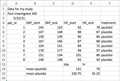
- Read in this file with the {readxl} package. Just for fun, try this see how this turns out with no additional arguments.
- Be sure to skip the problematic non-data first few rows
- Be sure to exclude the problematic non-data calculations below the table.
Solution to Challenge 1: paulolol.xlsx
## # A tibble: 8 × 6
##   pat_id SBP_start SBP_end HR_start HR_end treatment
##    <dbl>     <dbl>   <dbl>    <dbl>  <dbl> <chr>
## 1      1       145     120       92     78 paulolol
## 2      2       147     148       88     87 placebo
## 3      3       158     139       96     80 paulolol
## 4      4       167     166       87     88 placebo
## 5      5       154     131       84     72 paulolol
## 6      6       178     177       99     97 placebo
## 7      7       151     134      101     86 paulolol
## 8 8 149 148 92 93 placebo- Our intrepid Investigator has inserted a chart in place of his data table on sheet 1, and moved the data table to a 2nd sheet named ‘data’, and placed in the top left corner, at the suggestion of his harried statistician, in a new file with the path of ’data/paulolol2.xlsx”
- Try reading this file in with read_excel()
- read the help file
help(read_excel)to figure out how to read in the data from this excel file.
Solution to Challenge 2: paulolol2.xlsx
## # A tibble: 8 × 6
##   pat_id SBP_start SBP_end HR_start HR_end treatment
##    <dbl>     <dbl>   <dbl>    <dbl>  <dbl> <chr>
## 1      1       145     120       92     78 paulolol
## 2      2       147     148       88     87 placebo
## 3      3       158     139       96     80 paulolol
## 4      4       167     166       87     88 placebo
## 5      5       154     131       84     72 paulolol
## 6      6       178     177       99     97 placebo
## 7      7       151     134      101     86 paulolol
## 8      8       149     148       92     93 placebo
5.13 Future forms of data ingestion
- https://www.datacamp.com/community/tutorials/r-data-import-tutorial?utm_source=adwords_ppc&utm_campaignid=1658343521&utm_adgroupid=63833880415&utm_device=c&utm_keyword=%2Bread%20%2Bdata%20%2Br&utm_matchtype=b&utm_network=g&utm_adpostion=&utm_creative=469789579368&utm_targetid=aud-392016246653:kwd-309793905111&utm_loc_interest_ms=&utm_loc_physical_ms=9016851&gclid=Cj0KCQjwxJqHBhC4ARIsAChq4auwh82WzCiJsUDzDOiaABetyowW0CXmTLbUFkQmnl1pn4Op9xcCcdQaAhMWEALw_wcB
- reading data from the web with readr
- reading data from Google Sheets with {googlesheets}
- reading data from REDCap, and tidying
- reading data from web tables with rvest