Chapter 4 Introduction to Reproducibility

One of the major goals of this book is to help medical researchers make their research projects reproducible. This means being able to take the original raw data, and replicate each step of the data cleaning and analysis to produce the same end products, including tables, figures, and the full manuscript.

This requires:

• Robust sharing of data, materials, software, and code
• Documenting the data collection and data analysis processes
• Using authenticated biomaterials, and validated measurement instruments
• Using valid statistical methods and study design
• Pre-registration of studies, including detailed protocols and statistical plans, to avoid p-hacking and HARK-ing (Hypothesizing After the Results are Known (aka post-hoc analyses))
• Publishing (even if only on MedRxiv, or in the American Journal of Gastroenterology Black Issue) well-designed negative studies

This book largely focuses on computational reproducibility, as this is rarely taught in medical training, and intense pressure to publish leads the untrained into dark practices.

4.1 First Steps to Research Reproducibility

4.1.1 Have a Plan

The first steps toward research reproducibility come in planning for reproducibility. This means having a clear design and statistical plan, proven methods of data collection and recording, and preserving your raw data in a secure, locked state.

4.1.2 Treat Your Raw Data Like Gold

Largely because you spend a lot of money (often other peoples’ $$grant$$ money) and your own time (and the time of the people who work for you on the studies) in collecting it - you and others have invested a lot of gold to collect this. Once it is collected, it should be protected, backed up, and kept in a safe repository. Seriously consider having off-site backups for major projects to protect your data from local natural disasters. No one at Tulane expected Hurricane Katrina to destroy decades of research data. No one at NYU realized that the backup generators (in the basement) would be flooded by Hurricane Sandy. No one expects that their data and biosamples will be destroyed. But in an era (2022) when major natural disasters are increasing rapidly, it is important to plan for Black Swan events. Protect your research and protect your career.

4.1.3 Cleaning and Analyzing Your Data

There are a number of levels of reproducibility, and the following figure/meme illustrates these.

Levels of Reproducibility

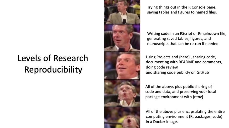
While an amusing meme, the image above does illustrate the arc of progress we hope to make as we move from ‘back of the envelope/Excel’ research to reproducible research. You don’t have to be making encapsulated research environments right away, but you can work up to that level.

Working in Excel, or any other point-and-click environment, is not fundamentally reproducible. There are multiple steps that are not recorded, calculations that are not transparent, and formulas that difficult to check (thus, forensic accounting is a growing field). Working in Excel leads to many, many errors, which have caused significant damage. Excel was never designed for research. It was designed for exploring data for small businesses, and it does not scale well.

going off on a tangent on the Perils of Excel, with examples

Working in a free, open-source coding language like R greatly eases the transition to reproducible research. It provides tools, accessible to anyone with an internet connection, to make science reproducible and transparent.

4.1.4 The First Level of Reproducibility

Working in the Console Pane in RStudio allows you to test code, trying out functions on your data. This is a good sandbox where you can do little harm, and is helpful when you are using a new package or function, and figuring out the syntax. You may need to get help for the function (?function_name), and it may take several iterations to get it to do what you want. You may jump over to a browser window to google something from RStudio Community, StackOverflow, or a good blog post to find an example.

You can even save the results (a table, a figure) to a folder with functions like this in a code chunk.

save(table, file = "table.csv")

ggsave(plot, filename = "figure1.jpg", device = "jpeg", width = 8, height = 5, units = "inches")

This is a good start, and your code is logged in the History, but it is not saved in a named file that you can go back to, and re-run. If your data changes, you have to start all over, and re-write the code. This is not very reproducible.

4.1.5 The Second Level of Reproducibility

You can bridge from the sandbox of the Console pane to reproducible, saved code. There are a couple of nice features in the History tab (top right in RStudio) to help you.

To get started, you need to Open a File to save your code in. As a default, we will start with RMarkdown files. In the RStudio menu, select ** File/New File/Rmarkdown… and give it a title, like “My First Analysis”. This will open a file in the RStudio Source pane (top left).

Note that this title (“My First Analysis”) is the title at the top of the resulting document, not the name of the file itself.

Once the file opens, you can see a header at the top, with Title, Author, Date, and Output Fields. This is called the YAML header, and it gives instructions for how the document will be processed to make a manuscript or HTML page. The YAML header is fenced with both an opening and a closing line of 3 dashes ---.

To save the file itself, you can use Cmd-S(Mac)/Ctrl-S(Windows), or click on the Save icon at the top of the file, then give it a filename, which is generally in lower case, with no numbers or spaces, and no punctuation except for underscores and hyphens. Each Rmarkdown filename ends with .Rmd

The first code chunk - the setup chunk - is provided for you in the Rmarkdown template, just below the YAML header. This is where you load packages, with the library(_packagename_) function. You want to load your packages at the beginning of the file, so that the functions and data from these packages are available later in the file.

Notice that code chunks are set off with 3 backticks at the beginning and end. The first set of backticks is followed by a letter r inside of curly braces, like this: {r}. This tells Rstudio that the following code will be in the R language.

The {r} can be followed by an (optional) chunk name (like setup), then a comma, and a number of (optional) code chunk options. Sometimes the code chunk options can get a bit ungainly, and you can enter them like comment lines at the top of the code chunk, before the code actually starts, using the hash-pipe marker, with commas between each option, like this:

```{r example}
#| echo = TRUE,
#| eval = FALSE
medicaldata::cytomegalovirus %>% 
  head()
```

You can insert new Code chunks with the green button that has a white letter C on it, and a plus sign at the top left corner of the button, at the top of the Source pane. When you click on it, R is the first option, but other computer languages are available.

Often, when you are writing code, you will start with experiments in the Console pane (lower left). Each time it does not quite work, you can use the up-arrow to pull down the most recent entry, to edit it and try again.

Another helpful tip, if you want to find code that you ran a few steps ago, is to press the up arrow (and down arrow) a few times until you reach the code you want. If it was a while back, it may be helpful to enter the first few characters of the code, then use Cmd-UpArrow(Mac) or Ctrl-UpArrow(Win) use those characters to search through the history for what you want.

Another helpful tip is that when you are running a function, and trying to get all the arguments set properly (between the parentheses), you can ask RStudio to prompt you for the remaining arguments. If you have your cursor between the parentheses, you can press the tab key and RStudio will give you a list of possible arguments for the function. You can select one and set it to an appropriate value. After each argument is set, you can enter a comma, and press the tab key again to get the list of arguments for that function.

Try this out with the code chunk named cars in the Rmarkdown template. Insert your cursor after the word cars, before the close-parenthesis. Add a comma, then press the tab key. Set the digits argument to 2 or 5, then run the chunk (with the green arrow to the right) to see how the results change.

Once you have worked out how to run a bit of code in the Console, it is helpful to click on the History tab. You will see all of your prior attempts.

You can scroll up and down to find a working version of your code, and then click on buttons at the top of the window to send that line of code to either the - Console, or - Source pane

If your cursor was in the code chunk you want in the Rmarkdown file, your working version will be copied from the History to your code chunk.

Rmarkdown is designed to be literate code, with the default for headers and explanatory text, as shown in the Rmarkdown template, and a few code chunks inserted into the manuscript where needed.

Note that there are three other options of document types to save your reproducible code. - R script (.R) - R notebook (.nb) - Quarto document (*.qmd)

An R script just has code, with minimal explanation or documentation. This is limiting for reproducible research. You can add a few comments, but it is a long way from an understandable workflow or a manuscript.

An R notebook is a hybrid, with an R script and HTML output as an option.

The Rmarkdown documemt can be processed (knitted) to create Word documents, pdfs, Poerpoint presentations, and HTML web pages.

Quarto documents are a newer version of code documentation that has a lot of the function of Rmarkdown.

4.2 The Foundations of Reproducibility

To make your data cleaning and analysis reproducible, you depend on several layers of reproducibility, several of which are out of your control.

1. The hardware that you work on - think of this as the foundation. We expect and assume that the hardware will not make computational errors, and will not differ between an Intel chip vs. an AMD chip vs. a Mac M-series chip. This is usually true, but the Pentium FDIV bug is a famous example of a hardware error that caused problems for a small number of users, but caused huge reputational damage to Intel, which changed their approach to hardware testing. The hardware is the foundation of reproducibility.

2. The operating system that you work on. There are differences between Windows, Linux, Mac, and other OSes. Hopefully these differences do not change computational results.

3. The statistical programming language that you use. R is a programming language, and it is open source, so it is constantly being updated and tested by the public. The R Foundation has a commitment to reproducibility and the R Core team works hard to ensure that computational results are reproducible across versions of R. There are slight differences between R, SAS, Stata, and other statistical programming languages, which can affect outputs, usually based on slightly different defaults in particular computations.

It is important to be aware of these, and when in doubt, to check the CAMIS project, which has a goal “to demystify conflicting results between software and to help ease the transitions to new languages by providing comparison and comprehensive explanations.” These differences are usually small, and can often be resolved by choosing a different computational option in the function arguments.

4. The R version that you are using. R is constantly being updated, and the R Foundation has a commitment to reproducibility and the R Core team works hard to ensure that the results are reproducible across versions of R. But it is still possible that switching from R 3.1 to R 5.2 will produce different results.

5. The R packages and versions that you use. R is a package-based language, and the packages are constantly being updated. Each package developer is aiming for reproducibility, but they may make major breaking changes between package versions that can make your code fail or produce different output. Each package team works hard to ensure that the results are reproducible across versions. But it is still possible that switching from {dplyr} 1.0.0 to {dplyr} 2.0.0 will cause your code to fail (most often) or produce different results (rarely). You can protect your projects from this problem by using the {renv} package, which will save the versions of the packages you are using in a project-specific library. This is a good practice for reproducibility, and is especially important when you are working on a project with multiple collaborators.

6. Your code. This is the most important part of reproducibility, and the part that you have the most control over. Your code should be well documented, and should be able to be run by someone else without any changes (including changes to paths, which may require the {here} package to work on different computers). Being able to produce the same results with the same data and code on any computer is the goal of reproducible research.

Future steps/goals in Reproducibility:

• building Projects in RStudio,
• using the {here} package for file paths
• documenting multiple code files in order with README
• saving interim clean/restructured data files
• backing up / collaborating / code sharing on GitHub
• code review with colleagues to check/test your analysis
• sharing deidentified data and code publicly
• preserving your project package environment with {renv}
• building an encapsulated coding environment with Docker and sharing on DockerHub