Chapter 23 Sample Size Calculations with {pwr}
When designing clinical studies, it is often important to calculate a reasonable estimate of the needed sample size. This is critical for planning, as you may find out very quickly that a reasonable study budget and timeline will be futile. Grant funding agencies will be very interested in whether you have a good rationale for your proposed sample size and timeline, so that they can avoid wasting their money.
Fortunately, the {pwr} package helps with many of the needed calculations. Let’s first install this package from CRAN, and load it with a library() function.
Remember that you can copy each code chunk to the clipboard, then paste it into your RStudio console (or a script) to edit and run it. Just hover your mouse pointer over the top right corner of each code chunk until a copy icon appears, then click on it to copy the code.
The {pwr} package has a number of functions for calculating sample size and power.
| Test | Sample Size Function |
|---|---|
| one-sample, two-sample, and paired t-tests | pwr.t.test() |
| two-sample t-tests (unequal sample sizes) | pwr.t2n.test() |
| two-sample proportion test (unequal sample sizes) | pwr.2p2n.test() |
| one-sample proportion test | pwr.p.test() |
| two-sample proportion test | pwr.2p.test() |
| two-sample proportion test (unequal sample sizes) | pwr.2p2n.test() |
| one-way balanced ANOVA | pwr.anova.test() |
| correlation test | pwr.r.test() |
| chi-squared test (goodness of fit and association) | pwr.chisq.test() |
| test for the general linear model | pwr.f2.test() |
Now that you have {pwr} up and running, we can start with a simple example.
23.1 Sample Size for a Continuous Endpoint (t-test)
Let’s propose a study of a new drug to reduce hemoglobin A1c in type 2 diabetes over a 1 year study period. You estimate that your recruited participants will have a mean baseline A1c of 9.0, which will be unchanged by your placebo, but reduced (on average) to 7.0 by the study drug.
You need to calculate an effect size (aka Cohen’s d) in order to estimate your sample size. This effect size is equal to the difference between the means at the endpoint, divided by the pooled standard deviation. Many clinicians can estimate the means and the difference, but the pooled standard deviation is not very intutitive. Sometimes you have an estimate from pilot data (though these tend to have wide confidence intervals, as pilot studies are small). In other circumstances, you can estimate a standard deviation for Hgb A1c from values from a large data warehouse. When you don’t have either of these, it can be helpful to start by estimating the range of values.
This is something that is intutitive, and experienced clinicians can do fairly easily. Just get a few clinicians in a room, and ask them for the highest and lowest values of HgbA1c that they have ever seen. You will quickly find a minimum and maximum that you can estimate as the range (in this case, let’s say 5.0 and 17.0 for min and max of Hgb A1c). This range divided by 4 is a reasonable rough estimate of the standard deviation. Remember that a normally distributed continuous value will have a 95% confidence interval that is plus or minus 1.96 standard deviations from the sample mean. Round this up to 2 for the full range, and you can see why we divide the range by 4 to get an estimate of the standard deviation.
In our case, the difference is 2 and the range/4 (estimate of SD) is 3. So our effect size (Cohen’s d) is 0.66. Plug in 0.66 for d in the code chunk below, and run this code chunk to get an estimate of the n in each arm of a 2 armed study with a two sample t-test of the primary endpoint.
pwr::pwr.t.test(n = NULL,
                sig.level = 0.05,
                type = "two.sample",
                alternative = "two.sided",
                power = 0.80,
                d = __)
We come up with 37.02 participants in each group to provide 80% power to detect a difference of 2 in HgbA1c, assuming a standard deviation of 3, using a two-sided alpha of 0.05. To conduct this study, assuming a 20% dropout rate in each arm, would require 37+8 subjects per arm, or 90 overall. At an enrollment rate of 10 per month, it will require 9 months to enroll all the participants, and 21 months (9 + 12 month intervention) to complete the data collection.
It is a very common mistake to look at the result for n, and assume that this is your total sample size needed. The n provided by {pwr} is the number per arm. You need to multiply this n by the number of arms (or in a paired analysis, by the number of pairs) to get your total n.
Another common mistake is to assume no dropout of participants. It is important to have a reasonable estimate (10-20% for short studies, 30-50% for long or demanding studies) and inflate your intended sample size by this amount. It is even better if you know from similar studies what the actual dropout rate was, and use this as an estimate (if there are similar previous studies). As a general rule, it is better to be conservative, and estimate a larger sample size, than to end up with p = 0.07.
Once you define your test type (the options are “two.sample”, “one.sample”, and “paired”), and the alternative (“two.sided”, “greater”, or “less”), four variables remain in a sample size and power calculation.
These are the remaining four arguments of the pwr.t.test() function. These are:
n
the significance level (sig.level)
the power
the effect size (Cohen’s d)
If you know any three of these, you can calculate the fourth. In order to do this, you set the one of these four arguments that you want to calculate equal to NULL, and specify the other 3. Imagine that we only have enough funds to run this study on 50 participants. What would our power be to detect a difference of 2 in Hgb A1c? You can set the power to NULL, and the n to 25 (remember that n is per arm), and run the chunk below.
pwr::pwr.t.test(n = __, # note that n is per arm
                sig.level = 0.05,
                type = "two.sample",
                alternative = "two.sided",
                power = __,
                d = 0.66)
We end up with 62.8% power, assuming no participant dropout (which is an extremely unlikely assumption). You can do the same thing, changing the NULL, to calculate an effect size or a significance level, if you have any need to.
In most cases, you are calculating a sample size, then realizing that you might not have that much money/resources. Then many calculate the power you would obtain given the resources you actually have. Let’s show a few more examples.
23.2 One Sample t-test for Lowering Creatinine
Eddie Enema, holistic healer, has proposed an unblinded pilot study of thrice-daily 2 liter enemas with “Eddie’s Dialysis Cleanser,” a proprietary mix of vitamins and minerals, which he believes will lower the serum creatinine of patients on the kidney transplant waiting list by more than 1.0 g/dL in 24 hours. The creatinine SD in this group of patients is 2.
The null hypothesis is < 1.0 g/dL. The alternative hypothesis is >= 1.0 g/dL.
Cohen’s d is 1.0 (the proposed change, or delta)/2 (the SD) = 0.5.
How many participants would Eddie Enema have to recruit to have 80% power to test this one-sample, one-sided hypothesis, with an alpha of 0.05?
Check each of the argument values and run the chunk below to find out.
pwr::pwr.t.test(n = NULL, # note that n is per arm
                sig.level = 0.05,
                type = "one.sample",
                alternative = "greater",
                power = 0.8,
                d = 0.5)
Fast Eddie would need to recruit slightly more than 26 participants (you always have to round up to get whole human participants) to have 80% power, assuming no dropout between the first and third enema, or before the blood draw 24 hours after baseline. Note that since this is an unblinded, one-sample study, The n in the results is multiplied by the number of arms (there is only 1 arm) to give you a sample size of 27.
A note about alpha and beta
alpha is described as the type I error, or the probability of declaring significant a difference that is not truly significant. We often use a two-sided alpha, which cuts the region of significance in half, and distributes it to both tails of the distribution, allowing for both significant positive and negative differences. Alpha is commonly set at 0.05, which works out to 0.025 on each tail of the distribution with a two-tailed alpha.
beta is the power, or (1- the risk of type II error). Type II error is the probability of missing a significant result and declaring it nonsignificant after hypothesis testing. Power is often set at 80%, or 0.8, but can be 90%, 95%, or 99%, depending on how important it is not to miss a significant result, and how much money and time you have to spend (both of which tend to increase N and power).
There is often an important tradeoff between type I and type II error. Things that decrease type II error (increase power) like spending more time and money for a larger N, will increase your risk of type I error. Conversely, reducing your risk of type I error will generally increase your risk of type II error. You may be in situations in which you have to decide which type of error is more important to avoid for your clinical situation to maximize benefit and minimize harms for patients.
23.3 Paired t-tests (before vs after, or truly paired)
As you can see from the above example, you can use a before-after design to measure differences from baseline, and essentially convert a two-sample paired design (each participant’s baseline measurement is paired with their post-intervention measurement) to a single sample design based on the difference between the before and after values.
The before-after (or baseline-postintervention) design is probably the most common paired design, but occasionally we have truly paired designs, like when we test an ointment for psoriasis on one arm, and use a placebo or sham ointment on the other arm. When this is possible, through bilateral symmetry (this also works for eyedrops in eyes, or dental treatments), it is much more efficient (in the recruiting sense) than recruiting separate groups for the treatment and control arms.
To see the difference between two-sample and paired designs, run the code chunk below, for a two-sample study with a Cohen’s d of 0.8 and 80% power. Then change the type to “paired”, and see the effect on sample size.
pwr::pwr.t.test(n = NULL, # note that n is per arm
                sig.level = 0.05,
                type = "two.sample",
                alternative = "two.sided",
                power = 0.8,
                d = 0.8)
Note that this changes the needed sample size from 52 subjects (26 per arm) to 15 subjects (as there is only one participant needed each paired application of 2 study treatments, and n in this case indicates the number of pairs), though it would be wise to randomize patients to having the treatment on the right vs. left arm (to maintain the blind). This is a large gain in recruiting efficiency. Use paired designs whenever you can.
23.4 2 Sample t tests with Unequal Study Arm Sizes
Occasionally investigators want unbalanced arms, as they feel that patients are more likely to participate if they have a greater chance of receiving the study drug than the placebo. It is fairly common to use 2:1 or 3:1 ratios. Larger ratios, like 4:1 or 5:1, are thought to risk increasing the placebo response rate, as participants assume that they are on the active drug. This is somewhat less efficient in recruiting terms, but it may improve the recruiting rate enough to compensate for the loss in efficiency.
This requires a slightly different function, the pwr.t2n.test() function. Let’s look at an example below. Instead of n, we have n1 and n2, and we have to specify one of these, and leave the other as NULL. Or we can try a variety of ratios of n1 and n2, leaving the power set to NULL, and test numbers to produce the desired power.
We are proposing a study in which the expected reduction in systolic blood pressure is 10 mm Hg, with a standard deviation of 20 mm Hg. We choose an n1 of 40, and a power of 80%, then let the function determine n2.
pwr::pwr.t2n.test(n1 = 40,
                  n2 = NULL,
                sig.level = 0.05,
                alternative = "two.sided",
                power = 0.8,
                d = 0.5)
In this case, n2 works out to slightly over 153 in the drug arm, or nearly 4:1.
Calculating effect size, or Cohen’s d.
You can calculate the d value yourself. Or, you can make your life easier to let the {pwr} package do this for you. You can leave the calculation of the delta/SD to the program, by setting
d = (20-10)/20, and the program will calculate the d of 0.5 for you.
We can also round up the ratio to 4:1 (160:40) and determine the resulting power.
pwr::pwr.t2n.test(n1 = c(40),
                  n2 = c(160),
                sig.level = 0.05,
                alternative = "two.sided",
                power = NULL,
                d = 0.5)
This provides a power of 80.3%.
23.5 Testing Multiple Options and Plotting Results
It can be helpful to compare multiple scenarios, varying the n or the estimated effect size, to examine trade-offs and potential scenarios when planning a trial. You can test multiple particular scenarios by listing the variables in a concatenated vector, as shown below for n1 and n2.
pwr::pwr.t2n.test(n1 = c(40, 60, 80),
                  n2 = c(80, 120, 160),
                sig.level = 0.05,
                alternative = "two.sided",
                power = NULL,
                d = 0.5)
This provides 3 distinct scenarios, with 3 pairs of n1/n2 values, and the calculated power for each scenario.
You can also examine many scenarios, with the sequence function, seq(). For the sequence function, three arguments are needed:
from, the number the sequence starts from
to, the number the sequence ends at (inclusive)
by, the number to increment by
Note that the length of the sequences produced by seq() must match (or be a multiple of the other) if you are sequencing multiple arguments, so that there is a number for each scenario. If the lengths of the sequences are multiples of each other (8 and 4 in the example below), the shorter sequence (n2) will be silently “recycled” (used again in the same order) to produce a vector of matching length (8).
pwr::pwr.t2n.test(n1 = seq(from = 40, to = 75, by = 5),
                  n2 = seq(60, 120, 20),
                sig.level = 0.05,
                alternative = "two.sided",
                power = NULL,
                d = 0.5)
Sometimes it is helpful to look at multiple scenarios and plot the results. You can do this by leaving n = NULL, and plotting the results, as seen below. The null value will be varied across a reasonable range, and the results plotted, with an optimal value identified. The plot function will use ggplot2 if this package is loaded, or base R plotting if ggplot2 is not available. As you can see below, you can modify the ggplot2 plot of the results with standard ggplot2 functions.
results <- pwr::pwr.t2n.test(n1 = c(40),
                  n2 = NULL,
                sig.level = 0.05,
                alternative = "two.sided",
                power = 0.80,
                d = 0.5)

plot(results) +
  ggplot2::theme_minimal(base_size = 14) +
  labs(title = 'Optimizing Sample Size for my 2-Sided t test',
       subtitle = "Always Round up for Whole Participants, N = 194")
## Warning: Using `size` aesthetic for lines was deprecated in ggplot2 3.4.0.
## ℹ Please use `linewidth` instead.
## ℹ The deprecated feature was likely used in the pwr package.
## Please report the issue to the authors.
## This warning is displayed once every 8 hours.
## Call `lifecycle::last_lifecycle_warnings()` to see where this warning was
## generated.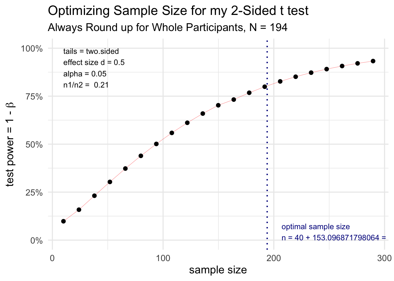
Note that the results object is a list, and you can access individual pieces with the dollar sign operator, so that `results$n1` equals 40, and `results$n2` equals 153.
You can examine the components of the results object in the Environment pane in RStudio. You can use these in inline R expressions in an Rmarkdown document to write up your results. Remember that each inline R expression is wrapped in backwards apostrophes, like `r code` (using the character to the left of the 1 key on the standard US keyboard), and starts with an r to let the computer know that the incoming code is written in R. This helps you write up a sentence like the below for a grant application:
Using an estimated effect size of 0.5, with a two-sided alpha of 0.05, we calculated that for 40 participants in group 1, 153.0968718 participants would be needed in group 2 to produce a power of 0.8.
When you knit an Rmarkdown file with these inline R expressions, each will be automatically converted to the result number and appear as standard text.
23.6 Your Turn
Try calculating the sample size or power needed in the continuous outcome scenarios below. See if you can plot the results as directed by editing the code chunks.
23.6.1 Scenario 1: FEV1 in COPD
You want to increase the FEV1 (forced expiratory volume in 1 second) of patients with COPD (chronic obstructive pulmonary disease) by 10% of predicted from baseline using weekly inhaled stem cells vs. placebo. Unfortunately, the standard deviation of FEV1 measurements is 20%. You want to have 80% power to detect this difference, with a 2-sided alpha of 0.05, with equal n in each of the two arms. Fill in the blanks in the code chunk below to calculate the sample size needed (n x number of arms). Remember that the effect size (Cohen’s d) = change in endpoint (delta)/SD of the endpoint.
pwr::pwr.t.test(n = __, # note that n is per arm
                sig.level = __,
                type = "__",
                alternative = "__",
                power = __,
                d = __)
You should get 128 participants (assuming no dropout) from 64 per arm. Cohen’s d is 10/20 = 0.5. It can be tricky to keep the type of “two.sample” and the alternative of “two.sided” straight. But you can do this!
23.6.2 Scenario 2: BNP in CHF
You want to decrease the BNP (brain natriuretic protein) of patients with CHF (congestive heart failure) by 300 pg/mL from baseline with a new oral intropic agent vs. placebo. BNP levels go up during worsening of heart failure, and a variety of effective treatments lower BNP, which can function as surrogate marker in clinical trials. The standard deviation of BNP measurements is estimated at 350 pg/mL. You want to have 80% power to detect this difference, with a 2-sided alpha of 0.05, with equal n in each of the two arms. Also consider an alternative scenario with a change in BNP of only 150 pg/mL. Remember that the effect size (Cohen’s d) = change in endpoint (delta)/SD of the endpoint. Fill in the blanks in the code chunk below (2 scenarios) to calculate the sample size needed (n x number of arms) for both alternatives.
pwr::pwr.t.test(n = __, # note that n is per arm
                sig.level = __,
                type = "two.__",
                alternative = "two.__",
                power = __,
                d = __/__)

pwr::pwr.t.test(n = __, # note that n is per arm
                sig.level = __,
                type = "two.__",
                alternative = "two.__",
                power = __,
                d = __/__)
You should get 46 participants (assuming no dropout) from 23 per arm x 2 arms, or 174 participants (87x2) with the alternative effect size. The effect size (Cohen’s d) is 300/350 = 0.86 in the original, and 150/350 (0.43) in the alternative effect.
Note that you can let R calculate the Cohen’s d - just type in 300/350 and 150/350, and R will use these as values of d.
23.6.3 Scenario 3: Barthel Index in Stroke
You want to increase the Barthel Activities of Daily Living Index of patients with stroke by 25 points from baseline with an intensive in-home PT and OPT intervention vs. usual care (which usually increases BADLI by only 5 points). You roughly estimate the standard deviation of Barthel index measurements as 38. You want to have 80% power to detect this difference, with a 2-sided alpha of 0.05, with equal n in each of the two arms. You want to consider multiple possible options for n, and plot these for a nice figure in your grant application. Fill in the blanks in the code chunk below to calculate and plot the sample size needed (n x number of arms).
results <- pwr::pwr.t.test(n = __, # note that n is per arm
                sig.level = __,
                type = "two.__",
                alternative = "two.sided",
                power = __,
                d = __ )
plot(results)
You should get an optimal sample size of 116 participants (assuming no dropout) from 58 per arm x 2 arms, with a nice plot to show this in your grant proposal. The effect size (Cohen’s d) is (25-5)/38 = 0.526.
23.7 Sample Sizes for Proportions
Let’s assume that patients discharged from your hospital after a myocardial infarction have historically received a prescription for aspirin 80% of the time. A nursing quality improvement project on the cardiac floor has tried to increase this rate to 95%. How many patients do you need to track after the QI intervention to determine if the proportion has truly increased?
the null hypothesis is that the proportion is 0.8
the alternative hypothesis is that the proportion is 0.95.
For this, we need the pwr.p.test() function for one proportion.
We will also use a built-in function of {pwr}, the ES.h() function, to help us calculate the effect size. This function takes our two hypothesized proportions and calculates an effect size with an arcsine transformation.
pwr.p.test(h = ES.h(p1 = 0.95, p2 = 0.80),
           n = NULL,
           sig.level = 0.05,
           power = 0.80,
           alternative = "greater")
##
## proportion power calculation for binomial distribution (arcsine transformation)
##
## h = 0.4762684
## n = 27.25616
## sig.level = 0.05
## power = 0.8
## alternative = greaterWe need to evaluate at least the next 28 patients discharged with MIs to have 80% power to test this one-sided hypothesis.
A note about test sided-ness and publication.
Frequently in common use, you may only be focused on an increase or decrease in a proportion or a continuous outcome, and a one-sided test seems reasonable. This is fine for internal use or local quality improvement work.
However, for FDA approval of a drug, for grant applications, or for journal publications, the standard is to always use two-sided tests, being open to the possibility of both improvement or worsening of the outcome you are studying. This is important to know before you submit a grant application, a manuscript for publication, or a dossier for FDA approval of a drug or device.
23.8 Sample size for two proportions, equal n
For this, we need the pwr.2p.test() function for two proportions.
You want to calculate the sample size for a study of a cardiac plexus parasympathetic nerve stimulator for pulmonary hypertension. You expect the baseline one year mortality to be 15% in high-risk patients, and expect to reduce this to 5% with this intervention. You will compare a sham (turned off) stimulator to an active stimulator in a 2 arm study. Use a 2-sided alpha of 0.05 and a power of 80%. Copy and edit the code chunk below to determine the sample size (n, rounded up) per arm, and the overall sample size (2n) fo the study.
We need to enroll at least 67 per arm, or 134 overall.
Dichotomous endpoints are generally regarded as having greater clinical significance than continuous endpoints, but often require more power and sample size (and more money and time). Most investigators are short on money and time, and prefer continuous outcome endpoints.
23.9 Sample size for two proportions, unequal arms
For this, we need the pwr.2p2n.test() function for two proportions with unequal sample sizes.
Imagine you want to enroll class IV CHF patients in a device trial in which they will be randomized 3:1 to a device (vs sham) that restores their serum sodium to 140 mmol/L and their albumin to 40 mg/dL each night. You expect to reduce 1 year mortality from 80% to 65% with this device. You want to know what your power will be if you enroll 300 in the device arm and 100 in the sham arm.
pwr.2p2n.test(h = ES.h(p1 = __, p2 = __),
           n1 = __,
           n2 = __,
           sig.level = __,
           power = __,
           alternative = "two.sided")
This (300:100) enrollment will have 84.6% power to detect a change from 15% to 5% mortality, with a two-sided alpha of 0.05.
23.10 Your Turn
Try calculating the sample size or power needed in the proportional outcome scenarios below. See if you can plot the results as directed by editing the code chunks.
23.10.1 Scenario 1: Mortality on Renal Dialysis
You want to decrease the mortality of patients on renal dialysis, which averages 20% per year in your local dialysis center. You will randomize patients to a bundle of statin, aspirin, beta blocker, and weekly erythropoietin vs. usual care, and hope to reduce annual mortality to 10%. You want to have 80% power to detect this difference, with a 2-sided alpha of 0.05, with equal n in each of the two arms. Fill in the blanks in the code chunk below to calculate the sample size needed (n x number of arms).
You always round up first (to whole participants per arm), then multiply by the number of arms. You will need a minimum of 98 per arm, for a total of 196 participants needed to complete the trial.
23.10.2 Scenario 2: Intestinal anastomosis in Crohn’s disease
You want to decrease 1-year endoscopic recurrence rate in Crohn’s disease from 90% to 70%. A local surgeon claims that his new “slipknot anastomosis” technique will accomplish this, by reducing colonic backwash and thereby, reducing endoscopic recurrence. You want to have 80% power to detect this difference, with a 2-sided alpha of 0.05, with equal n in each of the two arms. Also consider an alternative, more conservative scenario with a endoscopic recurrence rate of 80% with the new method. Fill in the blanks in the code chunk below to calculate the sample size needed (n x number of arms) for both alternatives.
pwr.p.test(h = c(ES.h(p1 = 0.9, p2 = __)),
           n = NULL,
           sig.level = .05,
           power = __,
           alternative = "two.sided")

pwr.p.test(h = c(ES.h(p1 = __, p2 = __)),
           n = __,
           sig.level = __,
           power = .80,
           alternative = __)
With the originally claimed recurrence proportion of 70%, you will need 30 participants per arm, or 60 for the whole study. The more conservative estimate will require 98 subjects per arm, or 196 for the whole study.
23.10.3 Scenario 3: Metformin in Donuts
Your local endocrinologist has identified consumption of glazed donuts as a major risk factor for development of type 2 diabetes in your region. She proposes to randomize participants to glazed donuts spiked with metformin vs usual donuts, expecting to reduce the 1 year proportion of prediabetics with a HgbA1c > 7.0 from 25% to 10%. You want to have 80% power to detect this difference, with a 2-sided alpha of 0.05, with 2 times as many participants in the metformin donut arm. You want to consider multiple possible sample sizes (n = 25, 50, 75) for the control glazed donuts, with 2n (double the sample size in each scenario) for the metformin donuts group. Fill in the blanks in the code chunk below to calculate the resulting power for each of the three sample size scenarios.
pwr.2p2n.test(h = ES.h(p1 = __, p2 = __),
           n1 = seq(from = __, to = __, by = 25),
           n2 = seq(from = __, to = __, by = 50),
           sig.level = __,
           power = NULL,
           alternative = "two.sided")
You should get a power of 37.7% for the smallest n, 64.5% for n1=50/n2=100, and 81.4% for the largest n scenario.
23.16 Explore More
You can explore other examples here in the official {pwr} vignette.
Power calculations for more complex endpoints and study designs can be found in R packages listed in the Clinical Trials CRAN Task View here. Consider the packages {samplesize}, {TrialSize}, {clusterpower}, {CRTsize}, {cosa}, {PowerTOST}, {PowerUpR}, and which may be relevant for your particular analysis.
Two other helpful references are books:
Cohen, J. (1988). Statistical Power Analysis for the Behavioral Sciences (2nd ed.). LEA.
Ryan, T.P. (2013) Sample Size Determination and Power. Wiley.