Chapter 49 Using the {heemod} package to Evaluate Markov Models of Health Economic Strategies

This chapter is part of the Clinical Applications pathway.
Packages needed for this chapter include {heemod} and {tidyverse}. If you don’t have these packages installed, you can install them by copying the code chunk below and running it in your local RStudio session.

install.packages("heemod")
install.packages("tidyverse")

49.1 Why Health Economic Evaluation and Markov Models?

Short-term decision analysis for acute illness that is unlikely to recur or for which the outcome is known with certainty can be done using a decision tree with a limited number of branches. However, for chronic diseases with multiple possible outcomes, a Markov model is often used. A Markov model allows for many branches, and the transition between distinct health states which have different utilities and costs. A Markov model also allows for repeated cycles over time, and distinct probabilities of transitions to the other health states. It is particularly useful for modeling chronic diseases where patients may move between different health states over time. Analysing costs and outcomes in a Markov model can help policymakers or practitioners make decisions about healthcare strategies and interventions. It can help to identify the most cost-effective strategies, and to understand the trade-offs between different options.

49.2 Preparation for Modeling

To prepare for modeling, we need to define the following components:

Health States: The different stages of the disease or condition being modeled.
Utilities: The quality of life associated with each health state.
Transition Probabilities: The likelihood of moving from one health state to another over a given cycle time.
Costs: The costs associated with each health state and the interventions being evaluated.
Time Horizon: The time period over which the model will be run. Ocassionally new treatments or interventions (like GLP-1s for obesity) can change and disrupt the status quo, so that a model is often no longer applicable after 5-20 years, as the field has changed. This is often difficult to estimate, as the time horizon may be much longer than the time period over which the model is run. For example, a model for diabetes may have a time horizon of 20 years, but the model may only be run for 5 years. This is often done to allow for the possibility of new treatments or interventions being introduced in the future.
Discount Rate: The rate at which future costs and outcomes are discounted to present value. This is typically 3-5%, based on interest rates for savings accounts, which are often used as a benchmark for discounting future costs and outcomes. The discount rate reflects the time value of money, and the opportunity cost of investing in one strategy over another. A higher discount rate will reduce the present value of future costs and outcomes, while a lower discount rate will increase their present value. The standard rates may be wildly off for some patients, who may have a much higher or lower discount rate based on their individual circumstances. For example, a patient with a terminal illness may have a much higher discount rate, as they may not expect to live long enough to benefit from future costs and outcomes. Conversely, a patient with a chronic illness who is expected to live for many years may have a lower discount rate, as they may be more likely to benefit from future costs and outcomes.

An enormous amount of work and literature searching can go into collecting all of the data needed to run a Markov model. It can often take more time than building and running the model itself. Be sure to allocate a good bit of time to collecting (and referencing) all of the source data needed to run the model. This includes the transition probabilities, utilities, costs, and any other data needed to run the model. It is also important to consider the quality of the data being used, as this can have a significant impact on the results of the model. For example, if the transition probabilities are based on low-quality data, this can lead to inaccurate results and conclusions.
Relatively new fields may not have enough published data on costs and utilities to build a model. However, a new intervention or strategy in an existing field, with documented costs and utilities, is often a good opportunity for health economic modelinng using the existing data. For example, a new intervention for diabetes (GLP-1s) may have new data on costs and efficacy, and you can use existing data on diabetes to build a model for the new intervention. You can evaluate whether and when the costs of the new intervention will produce significant benefits to justify the cost if the intervention.

49.3 Health States

When studying a chronic disease, we can define a set of health states that represent the different stages of the disease. For example, in a Markov model for diabetes, we might have the following health states: - Healthy: The patient is healthy and has no complications. - Diabetes: The patient has diabetes but no complications. - Diabetes with Complications: The patient has diabetes and one or more complications. - Death: The patient has died from diabetes or its complications. It is important to define the health states clearly, as they will be used to model the transitions between different states over time. All health states should be mutually exclusive and collectively exhaustive, meaning that every possible state of the disease should be represented by one of the defined health states. Each health state will have associated costs and utilities, which will be used to calculate the overall cost-effectiveness of the different strategies being evaluated.

49.4 Utilities

Each health state can be assigned a utility value, which represents the quality of life associated with that state. Utility values are typically measured on a scale from 0 to 1, where 0 represents death and 1 represents perfect health. For example, we might assign the following utility values to the health states in our diabetes model:

Healthy: 1.0
Diabetes: 0.8
Diabetes with Complications: 0.5
Death: 0.0

The utilities assigned should be justified by evidence from the relevant literature or expert opinion. It is important to note that utility values can vary between different populations and settings, so it is important to consider the context in which the model will be used. These are often derived using Time Trade Off (TTO) or Standard Gamble (SG) methods, which are used to elicit preferences for different health states.

49.5 Transition Probabilities

The transition probabilities represent the likelihood of moving from one health state to another (or staying in the same health state in the next cycle) over a given cycle time. For example, in our diabetes model, we might have the following transition probabilities per year:

Healthy to Diabetes: 0.01
Diabetes to Diabetes with Complications: 0.05
Diabetes with Complications to Death: 0.10
Diabetes to Healthy: 0.02

Note that each of these implies that most patients will stay in the same health state for the next cycle, and the sum of the probabilities for each health state must equal 1.0. For example, if a patient is in the “Healthy” state, they have a 99% chance of remaining healthy in the next cycle, a 1% chance of developing diabetes, and a 0% chance of dying. Obviously, someone in the “Death” state cannot transition to any other state, so the probabilities for that state are all 0.0 except for the probability of staying dead, which is 1.0.

49.6 Costs

The cost of each proposed strategy can be estimated using a variety of methods, including:

Charges (which may be inflated)
Actual costs (which may be deflated)
The Red Book costs of drugs - often accessed through Micromedex
literature sources

Each cost should be adjusted from the date it was published to current day prices, by adjusting for inflation in the intervening years. This is often a bit inaccurate, and efforts should be made to obtain the most recent costs for the drugs and procedures being studied. These costs should be estimated on a one-time or yearly basis, depending on whether they are one-time costs (like a surgery) or ongoing costs (like a maintenance medication). Do not neglect any trailing costs (e.g., managing wound infections in 20% after surgery) associated with follow-up care.

49.6.1 Maintenance Health Care Costs

If there are health care costs associated with a particular health state, like blood sugar monitoring and drug costs in diabetes, these should also be estimated, usually on a yearly basis, using the same methods as above.

49.7 Cycle Time

The cycle time is the time period over which the model will be run. This can vary depending on the disease being studied and the time frame of interest. For example, in a diabetes model, we might choose a cycle time of one year, as this is a common time frame for diabetes management. The cycle time should be chosen based on the natural history of the disease and the time frame of interest.

49.8 Building Your Model and Calculating Outcomes

A decision analysis can be done by hand, or in Microsoft Excel, but the calculations in a Markov model are more complex, and tools like R and the {heemod} package are helpful. The {heemod} package provides a wide range of features for modeling complex health economic problems. It is important to note that the {heemod} package is not the only option available for building Markov models in R, but it is one of the most widely used and well-documented packages for this purpose available. The PDF of the paper can be found here.

library(heemod)
library(tidyverse)

49.9 A First Model

To get started, we will build a simple basic model with {heemod}. This model will be a simple Markov model with two health states: “Healthy” (health state A) and “Sick” (health state B). The model will simulate the transition of patients between these two states over a period of 10 years.

When building a Markov model the following steps must be performed:

Specify transition probabilities between states.
Specify values attached to states (costs, utilities, etc.).
Combine this information and run the model.

49.10 The Transition State Matrix

The probability to transition from one state to another during a time period is called a transition probability. The time period itself is called a cycle. We can build a table of tranisition probabilities, called a transition state matrix. The rows of the table represent the current state, and the columns represent the next state. The values in the table represent the probability of transitioning from the current state to the next state.

Transition state table
	A	B
A	1	2
B	3	4

When starting a cycle in state A (row A), the probability to still be in state A at the end of the cycle is found in colunm A (cell 1) and the probability to change to state B is found in column B (cell 2).

Similarly, when starting a cycle from state B (row B), the probability to be in state A or B at the end of the cycle are found in cells 3 or 4 respectively.

You can define the transition matrix in {heemod} with the function define_transition(). The function takes a matrix as input, and the matrix should be a square matrix with the same number of rows and columns.

We are aiming for:

	A	B
A	0.9	0.1
B	0.2	0.8

# Define the transition matrix
mat_trans <- define_transition(
  0.9, 0.1,
  0.2, 0.8
)

## No named state -> generating names.

Then print out

mat_trans

## A transition matrix, 2 states.
## 
##   A   B  
## A 0.9 0.1
## B 0.2 0.8

Which will label these as health state A and health state B, since we did not name the health states. You can also name the health states by using the define_transition() function with the states argument.

49.11 Attach Values to States

Now it is time to add costs and utilities to each health state. for this example, we will use the following arbitrary values:

State A has a cost of 1234 per cycle and an utility of 0.85.
State B has a cost of 4321 per cycle and an utility of 0.50.

state_A <- define_state(
  cost = 1234,
  utility = 0.85
)
state_A

## A state with 2 values.
## 
## cost = 1234
## utility = 0.85

and for state B

state_B <- define_state(
  cost = 4321,
  utility = 0.50
)
state_B

## A state with 2 values.
## 
## cost = 4321
## utility = 0.5

49.12 Combining Transitions and Values into A Model

Now we use the define_strategy() function to combine the transition matrix and the state values into a model. The define_strategy() function takes the transition matrix and the state values as arguments, and returns a strategy object that can be used to run the model.

# Define the strategy
strat <- define_strategy(
  transition = mat_trans,
  state_A,
  state_B
)

## No named state -> generating names.

49.13 Run the Model

Now we are ready to run the model. For our initial model, we will run it through 10 cycles (in this case, years). The run_model() function takes the strategy object and the number of cycles as arguments, and returns a model object that contains the results of the simulation. By default, tje model will run for 1000 persons beginning in the first health state (state A).

res_mod <- run_model(
  strat,
  cycles = 10,
  cost = cost,
  effect = utility
)

## No named model -> generating names.

We can view the results in the res-mod object. The run_model() function returns a list of results, including the total cost and total utility for each health state, as well as the number of patients in each health state at the end of the simulation.

res_mod

## 1 strategy run for 10 cycles.
## 
## Initial state counts:
## 
## A = 1000L
## B = 0L
## 
## Counting method: 'life-table'.
## 
##  
## 
## Counting method: 'beginning'.
## 
##  
## 
## Counting method: 'end'.
## 
## Values:
## 
##       cost  utility
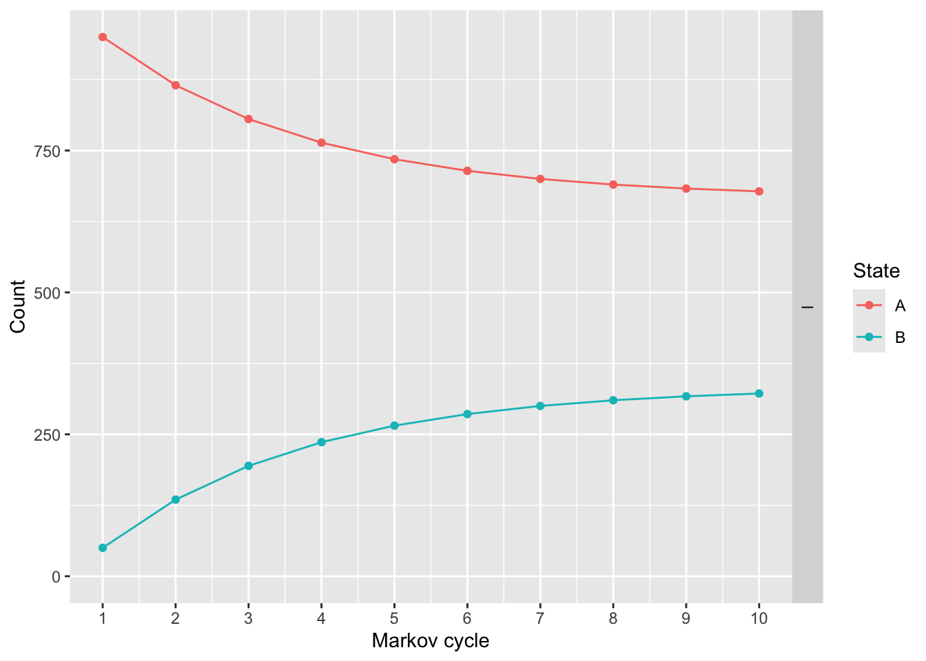
## I 19796856 7654.552

We can also plot the results. This shows how many people are in each health state by model cycle (year).

plot(res_mod)

We can modify these plots and make them prettier with ggplot2 syntax.

library(ggplot2)

plot(res_mod) +
  xlab("Time") +
  ylab("N") +
  theme_minimal() +
  scale_color_brewer(
    name = "State",
    palette = "Set1"
  )

## Scale for colour is already present.
## Adding another scale for colour, which will replace the existing scale.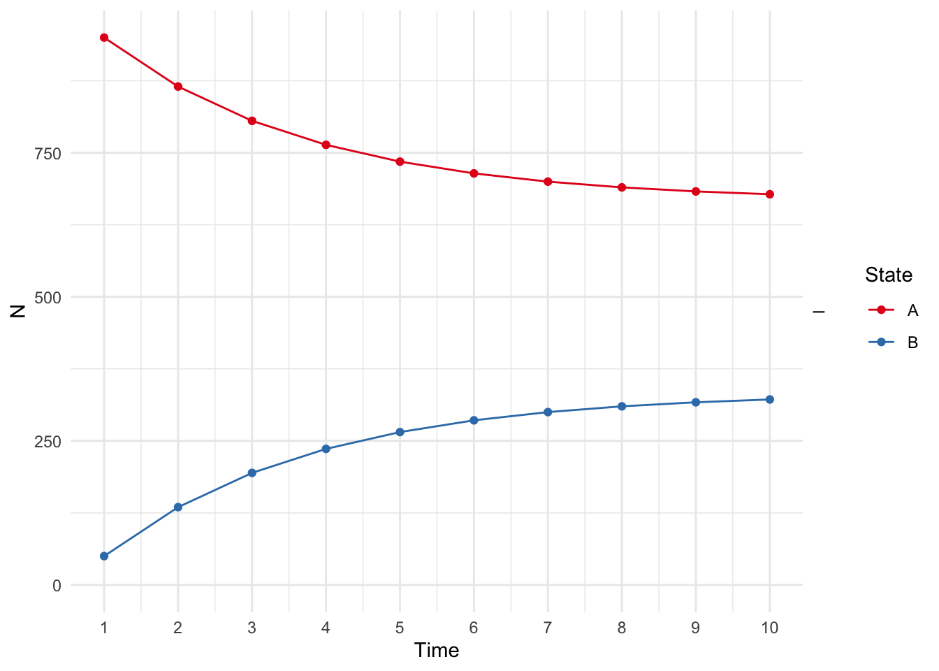

We can also use get_counts() and get_values() to get the number of patients in each health state and the total cost and utility for each health state at the end of the simulation. The get_counts() function returns a data frame with the number of patients in each health state at each cycle, and the get_values() function returns a data frame with the total cost and utility for each health state at each cycle.

# Get the counts#
get_counts(res_mod)

##    .strategy_names model_time state_names    count
## 1                I          1           A 950.0000
## 2                I          2           A 865.0000
## 3                I          3           A 805.5000
## 4                I          4           A 763.8500
## 5                I          5           A 734.6950
## 6                I          6           A 714.2865
## 7                I          7           A 700.0005
## 8                I          8           A 690.0004
## 9                I          9           A 683.0003
## 10               I         10           A 678.1002
## 11               I          1           B  50.0000
## 12               I          2           B 135.0000
## 13               I          3           B 194.5000
## 14               I          4           B 236.1500
## 15               I          5           B 265.3050
## 16               I          6           B 285.7135
## 17               I          7           B 299.9995
## 18               I          8           B 309.9996
## 19               I          9           B 316.9997
## 20               I         10           B 321.8998

# Get the values
get_values(res_mod)

##    model_time .strategy_names value_names        value
## 1           1               I        cost 1388350.0000
## 2           2               I        cost 1650745.0000
## 3           3               I        cost 1834421.5000
## 4           4               I        cost 1962995.0500
## 5           5               I        cost 2052996.5350
## 6           6               I        cost 2115997.5745
## 7           7               I        cost 2160098.3021
## 8           8               I        cost 2190968.8115
## 9           9               I        cost 2212578.1681
## 10         10               I        cost 2227704.7176
## 11          1               I     utility     832.5000
## 12          2               I     utility     802.7500
## 13          3               I     utility     781.9250
## 14          4               I     utility     767.3475
## 15          5               I     utility     757.1432
## 16          6               I     utility     750.0003
## 17          7               I     utility     745.0002
## 18          8               I     utility     741.5001
## 19          9               I     utility     739.0501
## 20         10               I     utility     737.3351

49.14 Your Turn

Let’s try to model the cost effectiveness of a combination treatment for HIV, when compared to monotherapy (this was modeled in 1997). We will consider four health states:

A: CD4 cells > 200 and < 500 cells/mm3;
B: CD4 < 200 cells/mm3, non-AIDS;
C: AIDS;
D: Death.

The costs for the drugs are as follows:

cost_zido <- 2278
cost_lami <- 2086

Go ahead and define the health states

state_A <- define_state(
  cost_health = discount(2756, .06),
  cost_drugs = discount(dispatch_strategy(
    mono = cost_zido,
    comb = cost_zido + cost_lami
  ), .06),
  cost_total = cost_health + cost_drugs,
  life_year = 1
)
state_A

## A state with 4 values.
## 
## cost_health = discount(2756, 0.06)
## cost_drugs = discount(...)
## cost_total = cost_health + cost_drugs
## life_year = 1

Now define the other health states. The costs for the drugs are the same for all health states, but the costs for the health states are different. The life years are also different for each health state. The discount rate of .06 stays the same for each health state.

State B health cost - 3052
State C health cost - 9007

State D (death) is easier to define:

state_D <- define_state(
  cost_health = 0,
  cost_drugs = 0,
  cost_total = 0,
  life_year = 0
)

The transition probabilities for monotherapy are as follows: | | A | B | C | D | |—–|—–|—–|—–|—–| | A | .721|.202 |.067 | .010| | B | 0 | .581| .407| .012| | C | 0 | 0 | .750| .250| | D | 0 | 0 | 0 | 1 |

Use the table above to define a transition matrix for monotherapy, mat_mono

mat_mono <- define_transition()

## No named state -> generating names.

The combination therapy has a RR f=of 0.509, and the define_transition function will accept the value C (the complement) for whatever is left over to reach a probability of 1. so this has the following transition probabilities:

	A	B	C	D
A	C	.202*rr	.067*rr	.010*rr
B	0	C	.407*rr	.012* rr
C	0	0	C	.250*rr
D	0	0	0	1

and you can code this with

rr <- .509

mat_comb <- define_transition(
  C, .202 * rr, .067 * rr, .010 * rr,
  0, C,       .407 * rr, .012 * rr,
  0, 0,       C,       .250 * rr,
  0, 0,       0,       1
)

## No named state -> generating names.

You can plot mat_mono and mat_comb to see the difference between the two transition matrices.

Now build the two strategies:

strat_mono <- define_strategy(
  name = "Mono",
  state_A,
  state_B,
  state_C,
  state_D,
  transition = mat_mono
)

## Error: object 'state_C' not found

You can build strat_comb, which is quite similar.

Then you can run the model as below.

res_mod <- run_model(
  mono = strat_mono,
  comb = strat_comb,
  cycles = 50,
  cost = cost_total,
  effect = life_year
)

## Error: object 'strat_mono' not found

You can then do a summary() of the res_mod, or plot it by strategy

plot(res_mod, type = "counts", panel = "by_strategy") +
  xlab("Time") +
  theme_bw() +
  scale_color_brewer(
    name = "State",
    palette = "Set1"
  )

## Scale for colour is already present.
## Adding another scale for colour, which will replace the existing scale.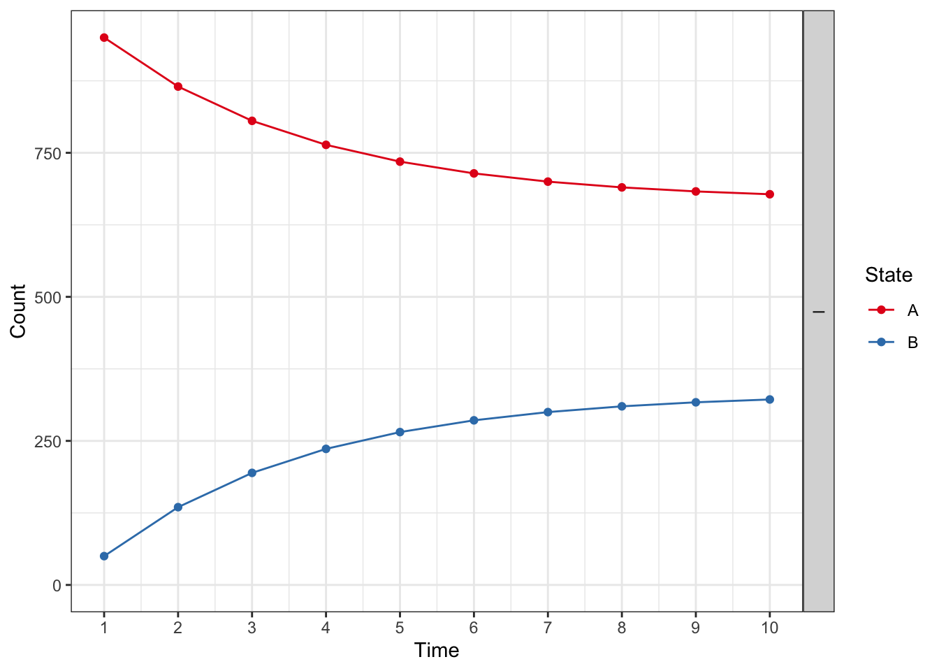

or plot by health state

plot(res_mod, type = "counts", panel = "by_state") +
  xlab("Time") +
  theme_bw() +
  scale_color_brewer(
    name = "Strategy",
    palette = "Set1"
  )

## Scale for colour is already present.
## Adding another scale for colour, which will replace the existing scale.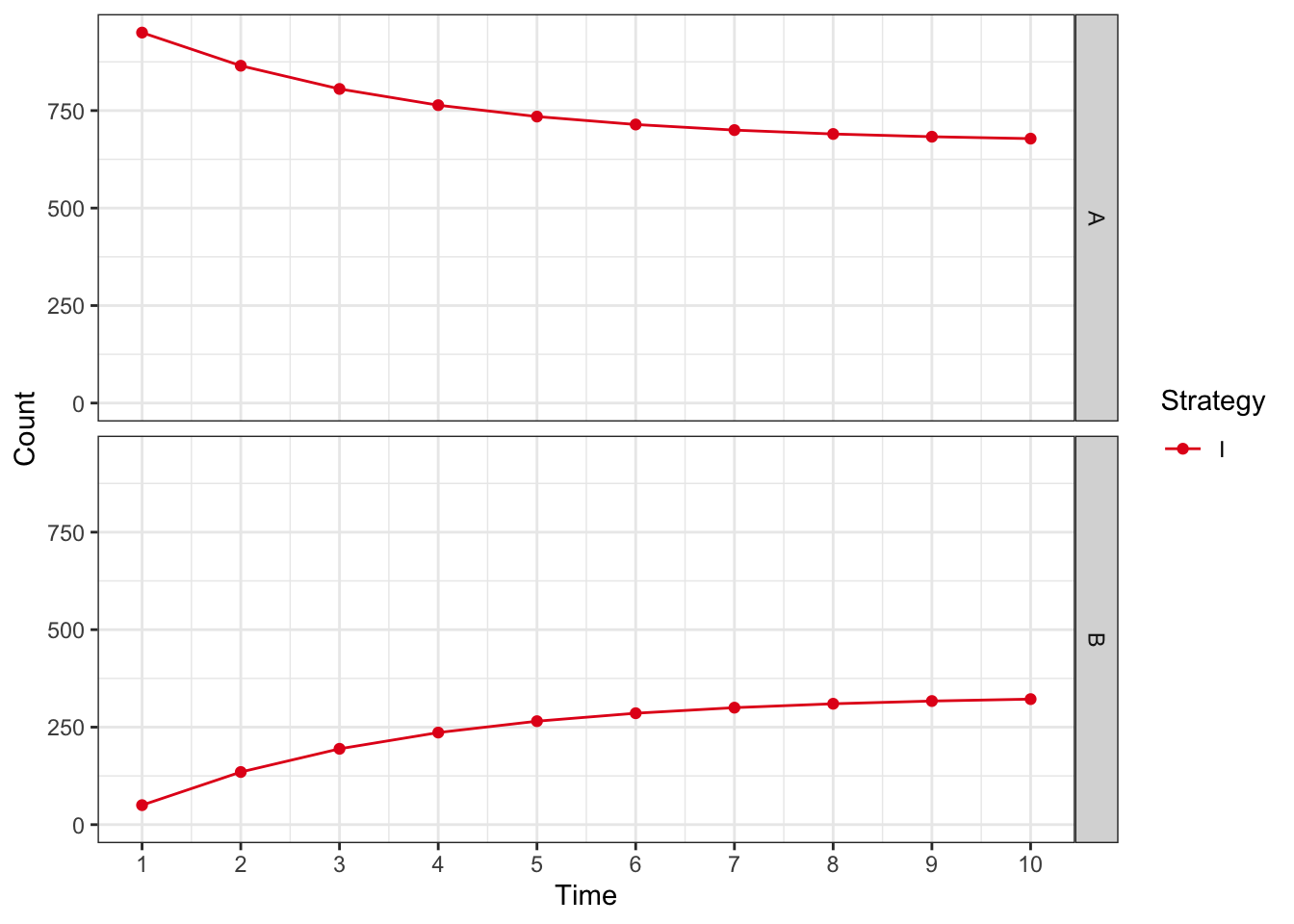

Work your way through this model, and explore the outputs. If you would like, a complete solution can be found below.

mat_mono <- define_transition(
  .721, .202, .067, .010,
  0,    .581, .407, .012,
  0,    0,    .750, .250,
  0,    0,    0,    1
)

## No named state -> generating names.

plot(mat_mono)

## Loading required namespace: diagram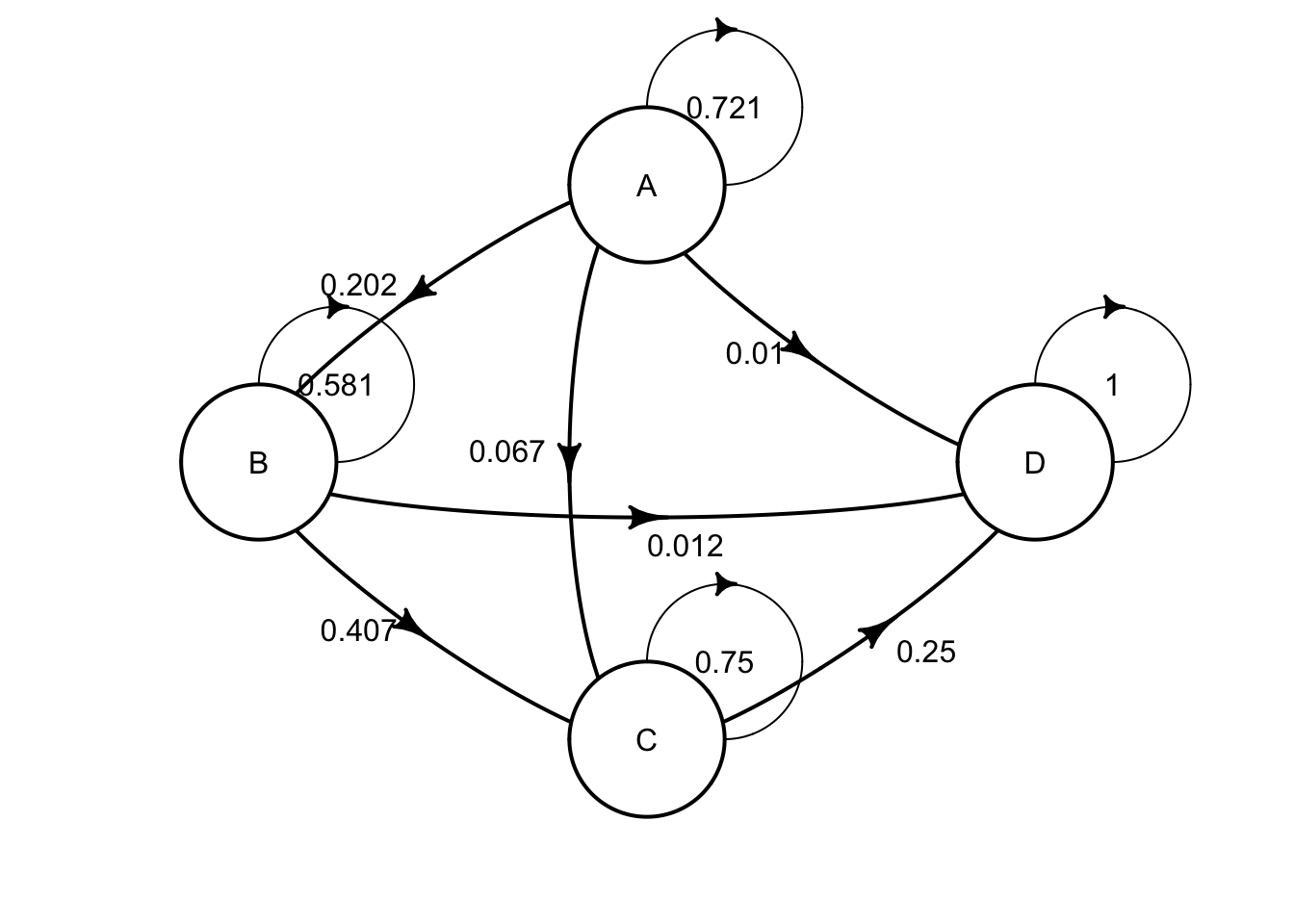

rr <- .509

mat_comb <- define_transition(
  C, .202 * rr, .067 * rr, .010 * rr,
  0, C,       .407 * rr, .012 * rr,
  0, 0,       C,       .250 * rr,
  0, 0,       0,       1
)

## No named state -> generating names.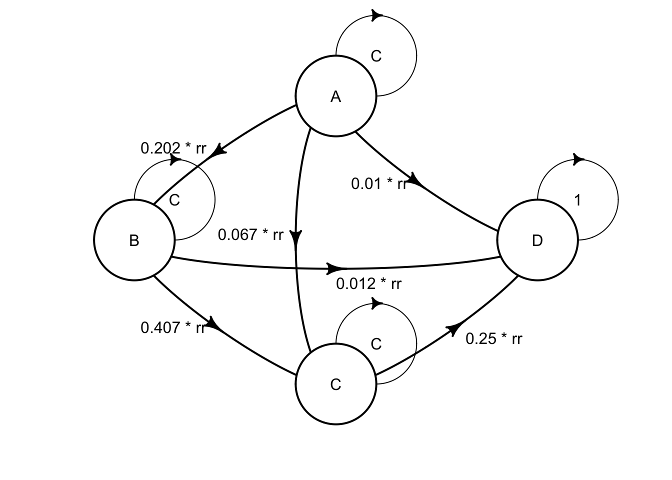

plot(mat_comb)

cost_zido <- 2278
cost_lami <- 2086

state_A <- define_state(
  cost_health = discount(2756, .06),
  cost_drugs = discount(dispatch_strategy(
    mono = cost_zido,
    comb = cost_zido + cost_lami
  ), .06),
  cost_total = cost_health + cost_drugs,
  life_year = 1
)

state_B <- define_state(
  cost_health = discount(3052, .06),
  cost_drugs = discount(dispatch_strategy(
    mono = cost_zido,
    comb = cost_zido + cost_lami
  ), .06),
  cost_total = cost_health + cost_drugs,
  life_year = 1
)
state_C <- define_state(
  cost_health = discount(9007, .06),
  cost_drugs = discount(dispatch_strategy(
    mono = cost_zido,
    comb = cost_zido + cost_lami
  ), .06),
  cost_total = cost_health + cost_drugs,
  life_year = 1
)
state_D <- define_state(
  cost_health = 0,
  cost_drugs = 0,
  cost_total = 0,
  life_year = 0
)

strat_mono <- define_strategy(
  transition = mat_mono,
  state_A,
  state_B,
  state_C,
  state_D
)

## No named state -> generating names.

strat_comb <- define_strategy(
  transition = mat_comb,
  state_A,
  state_B,
  state_C,
  state_D
)

## No named state -> generating names.

res_mod <- run_model(
  mono = strat_mono,
  comb = strat_comb,
  cycles = 50,
  cost = cost_total,
  effect = life_year
)

summary(res_mod,
  threshold = c(1000, 5000, 6000, 1e4)
)

## 2 strategies run for 50 cycles.
## 
## Initial state counts:
## 
## A = 1000L
## B = 0L
## C = 0L
## D = 0L
## 
## Counting method: 'life-table'.
## 
##  
## 
## Counting method: 'beginning'.
## 
##  
## 
## Counting method: 'end'.
## 
## Values:
## 
##      cost_health cost_drugs cost_total life_year
## mono    33891136   14870957   48762093  8585.843
## comb    48739757   44245091   92984848 17256.937
## 
## Net monetary benefit difference:
## 
##          1000     5000     6000    10000
## mono 35551.66 867.2847    0.000     0.00
## comb     0.00   0.0000 7803.809 42488.19
## 
## Efficiency frontier:
## 
## mono -> comb
## 
## Differences:
## 
##      Cost Diff. Effect Diff.    ICER Ref.
## comb   44222.75     8.671094 5100.02 mono

plot(res_mod, type = "counts", panel = "by_strategy") +
  xlab("Time") +
  theme_bw() +
  scale_color_brewer(
    name = "State",
    palette = "Set1"
  )

## Scale for colour is already present.
## Adding another scale for colour, which will replace the existing scale.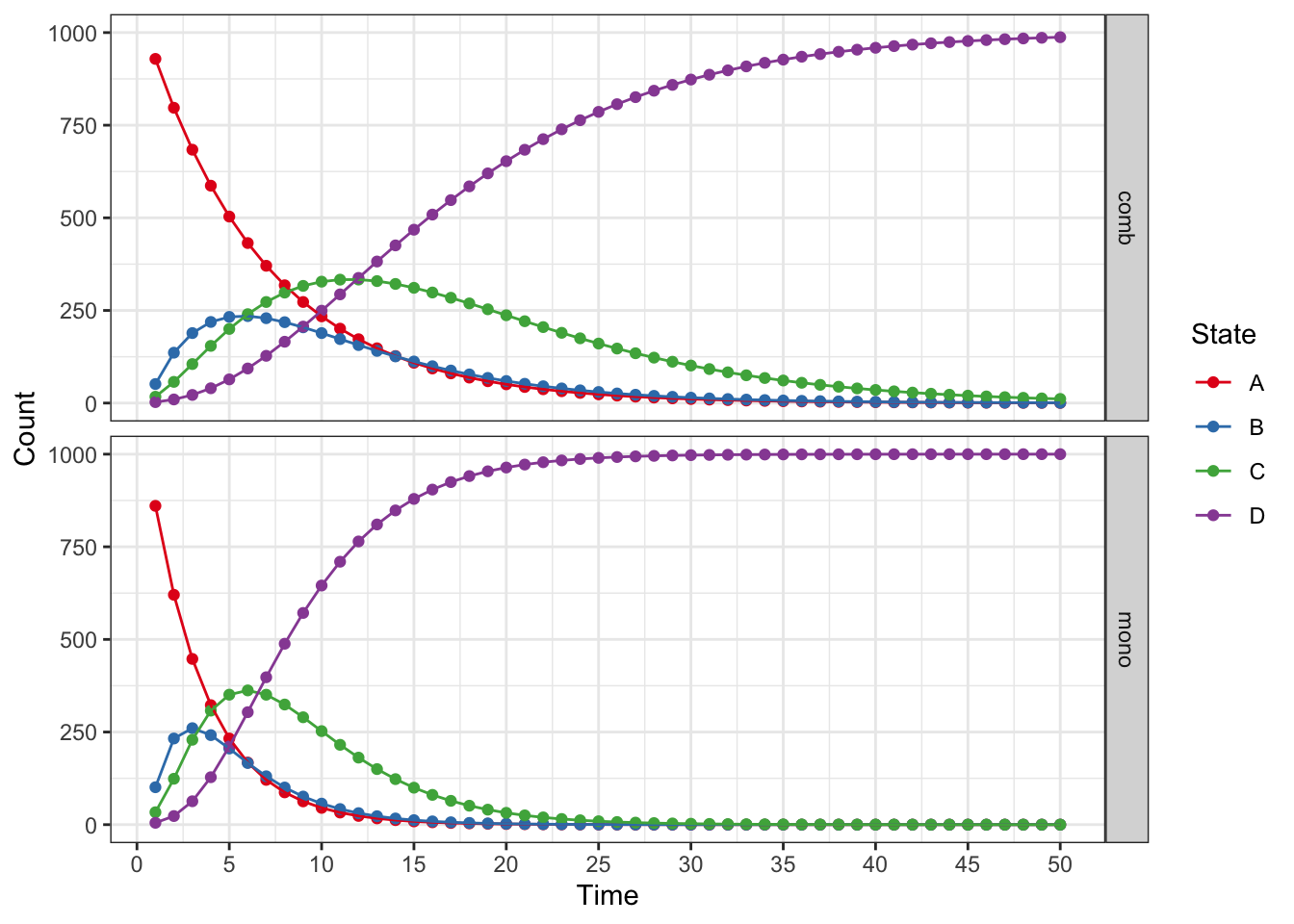

plot(res_mod, type = "counts", panel = "by_state") +
  xlab("Time") +
  theme_bw() +
  scale_color_brewer(
    name = "Strategy",
    palette = "Set1"
  )

## Scale for colour is already present.
## Adding another scale for colour, which will replace the existing scale.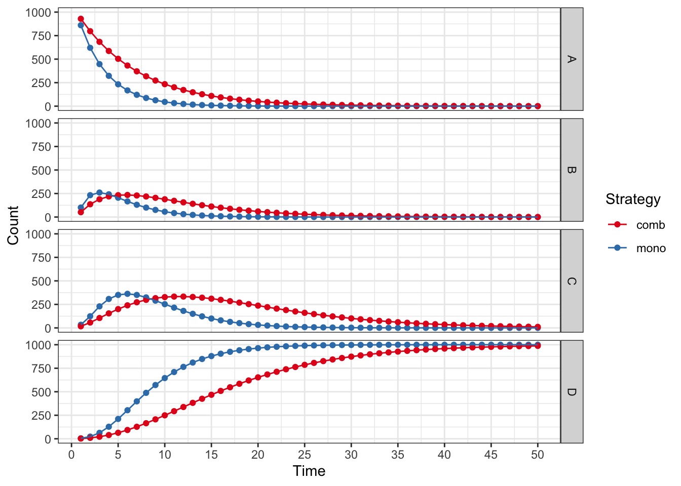

plot(res_mod,
  type = "values", panel = "by_value",
  free_y = TRUE
) +
  xlab("Time") +
  theme_bw() +
  scale_color_brewer(
    name = "Strategy",
    palette = "Set1"
  )

## Scale for colour is already present.
## Adding another scale for colour, which will replace the existing scale.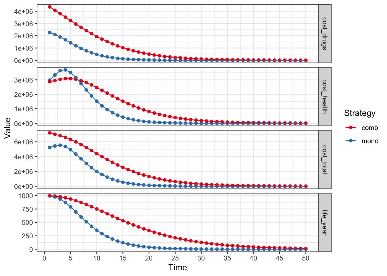

:::

49.14.1 Explore More Features

You can explore more features of {heemod} at several websites.
Start with the github.io website here. Check out all of the articles and vignettes.
The package and R Universe help files can be found here.
The full manual and help files can be found here.
Many videos about how to use {heemod} have been made. One good playlist (in mostly English / some Arabic) can be found here. This works through most of the examples in the {heemod} help and has a nice video on tornado plots for sensitivity analysis. A single video (without narration) can be found here

49.14.2 Explore Health Economics Beyond {heemod}

The {heemod} package is a great way to get started with health economic modeling in R. However, there are many other packages and resources available for those interested in this field.

A great resource is the R for Health Technology Assessment consortium (based in the UK), with a website found here. The R for HTA consortium website lists a number of R packages that are useful for health economic modeling, and this group holds an annual workshop (hybrid/online, inexpensive for students, low income country residents) in June along with a variety of training events and short courses. A number of talks (with slides) and a few tutorials can be found posted on the website.

If you want to go much deeper into this topic area, a whole series of handbooks on health economic evaluation from Oxford University Press can be found here.