Chapter 34 Introduction to R Markdown

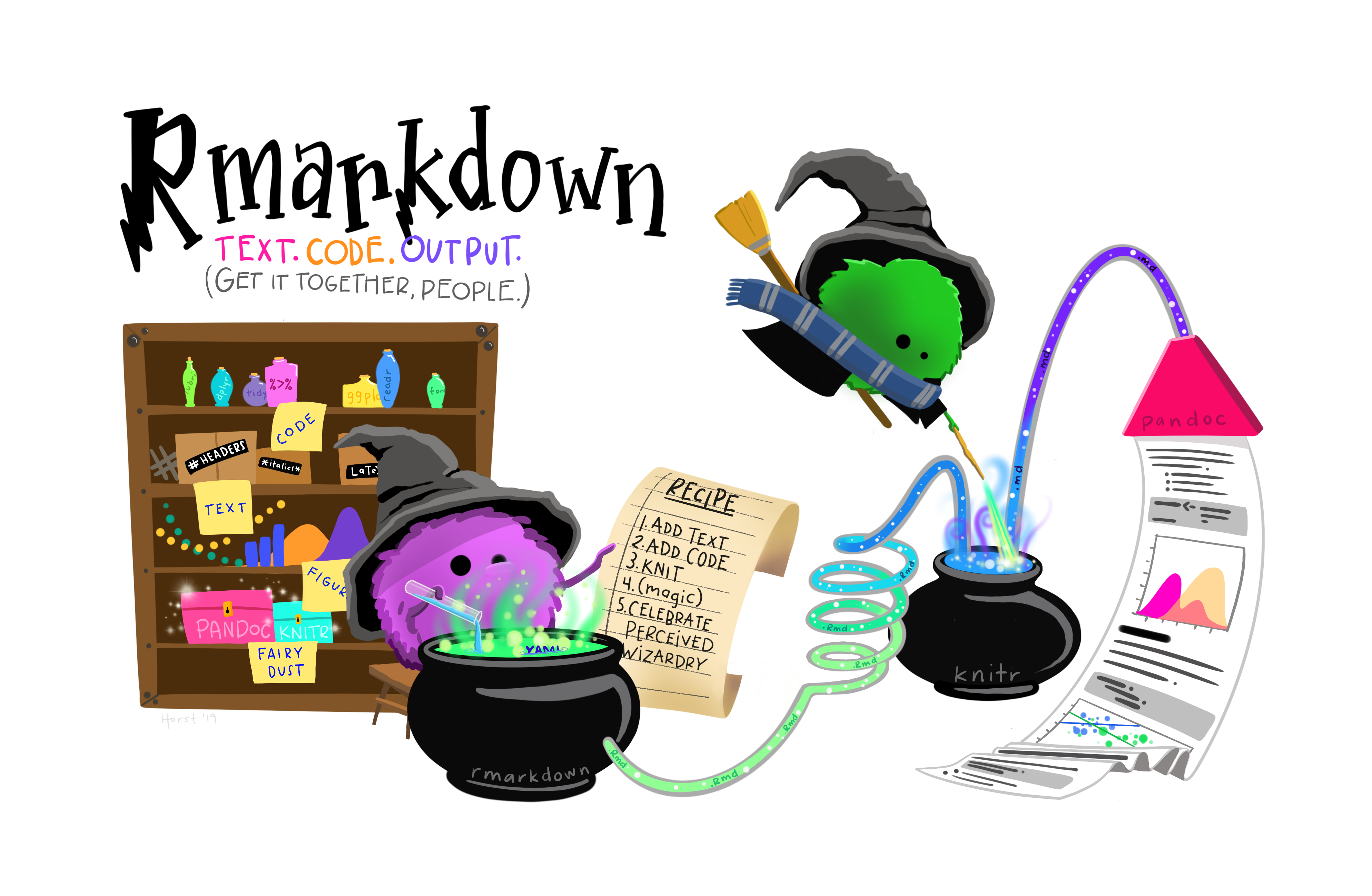
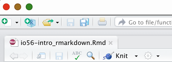
Rmarkdown Wizards, courtesy of Alison Horst

Rmarkdown is an authoring framework for creating a variety of data-driven documents reproducibly with R. This e-book is itself a set of RMarkdown documents, assembled with the {bookdown} package. In many ways, Rmarkdown is a critical package for the R ecosystem, as it is a key enabler of reproducible reports in many formats. RMarkdown is a simple formatting syntax that allows you to mix text and code to document data analysis, and author MS Word, MS Powerpoint, HTML, PDF, web dashboards, web apps, and poster documents. Rmarkdown documents are fully reproducible and support more than a dozen output formats. If your data changes, or you decide to change a part of your analysis, you can reproduce the entire (new version) of the document with a single click of the Knit button (You can also use Cmd/Ctrl+Shift+K). This button is found at the top of the top left pane in RStudio.

Knit button

When you click the Knit button a document will be generated that includes both text content as well as the output of any embedded R code chunks within the document. You can embed an R code chunk like this (which will run and produce output below. In this case, showing the contents of the covid_testing dataset.):

covid <- medicaldata::covid_testing
glimpse(covid)

## Rows: 15,524
## Columns: 17
## $ subject_id      <dbl> 1412, 533, 9134, 8518, 8967, 11048…
## $ fake_first_name <chr> "jhezane", "penny", "grunt", "meli…
## $ fake_last_name  <chr> "westerling", "targaryen", "rivers…
## $ gender          <chr> "female", "female", "male", "femal…
## $ pan_day         <dbl> 4, 7, 7, 8, 8, 8, 9, 9, 9, 9, 9, 9…
## $ test_id         <chr> "covid", "covid", "covid", "covid"…
## $ clinic_name     <chr> "inpatient ward a", "clinical lab"…
## $ result          <chr> "negative", "negative", "negative"…
## $ demo_group      <chr> "patient", "patient", "patient", "…
## $ age             <dbl> 0.0, 0.0, 0.8, 0.8, 0.8, 0.8, 0.8,…
## $ drive_thru_ind  <dbl> 0, 1, 1, 1, 0, 0, 1, 0, 1, 1, 1, 0…
## $ ct_result       <dbl> 45, 45, 45, 45, 45, 45, 45, 45, 45…
## $ orderset        <dbl> 0, 0, 1, 1, 1, 0, 1, 1, 1, 1, 0, 1…
## $ payor_group     <chr> "government", "commercial", NA, NA…
## $ patient_class   <chr> "inpatient", "not applicable", NA,…
## $ col_rec_tat     <dbl> 1.4, 2.3, 7.3, 5.8, 1.2, 1.4, 2.6,…
## $ rec_ver_tat     <dbl> 5.2, 5.8, 4.7, 5.0, 6.4, 7.0, 4.2,…

The Knit button (at the top of the top left pane of RStudio) runs
render("file.Rmd", output = document-type)
for you in a background (clean) session of R.

34.1 What Makes an Rmarkdown document?

An Rmarkdown document is a plain-text file with the *.Rmd file extension. It is composed of four types of content:

The YAML header (at the top), surrounded at top and bottom by 3 dashes (—)
Text narrative - the meat of your manuscript
Code chunks, surrounded at top and bottom by 3 back-ticks (```), and the chunk header in braces, like {r plot-figure}
- Note that the first code chunk is always named setup and is often used to load libraries and set up document options.
Inline code, which does calculations in your text to provide calculated values like means, medians, and p values.

This essentially provides an interface like a ‘lab notebook’ for data analysis. You can use code chunks to run the analysis, and text to document what you are doing in the analysis, how it worked, and interpret the results. When the analysis is ready, you can polish up your document to produce a final manuscript.

Code outputs, including tables and plots, are incorporated into the document.

You can choose to show or hide the code chunks in the final document with options in the chunk header, like:

{r, echo = FALSE} - runs code, but does not show it.
or
{r, echo = TRUE} - runs code and shows the code.

34.2 Trying out RMarkdown with a Mock Manuscript

Open up RStudio.

Start a new Project. Click - File - New Project… - Version Control > - Git >

Now paste the following into the Repository URL: box

https://github.com/higgi13425/rmd4medicine.git

add a directory name, like rmd4medicine
click on Create Project
Find the Files tab in the lower right quadrant.
Click to open the prep folder
Click to open the mockstudy_analysis.Rmd file.

This file should open in the top left quadrant of RStudio. If there are warnings at the top of the file that you need to install packages, click on the Install button.

34.3 Inserting Code Chunks

You can add code to your document to process your data and display results.

To insert a code chunk into your Rmarkdown document, click on the green +c button at the top center of the top left pane in RStudio.

The dropdown menu will allow you to choose R code or several other computer languages, For now, click on R.

This inserts a gray code chunk, which starts and stops with 3 back-ticks. The starting back-ticks are followed by braces containing a lower-case r, designating what follows as R code.

You can name your individual code chunks with specific names, based on what they do. You can click to the right of the lower-case r, before the closing brace, and add a space, then a name for the code chunk. If the chunk name contains multiple words, connect these with hyphens, as in the code chunk below. Avoid spaces, periods, and underscores in chunk names.

head(covid)

## # A tibble: 6 × 17
##   subject_id fake_first_name fake_last_name gender pan_day
##        <dbl> <chr>           <chr>          <chr>    <dbl>
## 1       1412 jhezane         westerling     female       4
## 2        533 penny           targaryen      female       7
## 3       9134 grunt           rivers         male         7
## 4       8518 melisandre      swyft          female       8
## 5       8967 rolley          karstark       male         8
## 6      11048 megga           karstark       female       8
## # ℹ 12 more variables: test_id <chr>, clinic_name <chr>,
## #   result <chr>, demo_group <chr>, age <dbl>,
## #   drive_thru_ind <dbl>, ct_result <dbl>, orderset <dbl>,
## #   payor_group <chr>, patient_class <chr>,
## #   col_rec_tat <dbl>, rec_ver_tat <dbl>

34.3.1 Code Chunk Icons

You may have noticed 3 small icons at the top right of each code chunk. From left to right, these are a (settings) gear, a downward arrowhead with a green baseline (run all of the preceding chunks), and a rightward (run) arrow. Check these out and experiment with them.

Code Chunk Icons
Icon	Uses
Settings Gear	Allows you to Name the code chunk Set options for this chunk
Run Chunks Above (down arrow)	Runs all of the preceding code chunks, including the setup chunk
Run Chunk (rightward arrow)	Runs the entire current chunk

34.4 Including Plots

You can also embed plots using code chunks, for example:

covid %>% 
  ggplot() +
  aes(x = pan_day, y = ct_result) +
  geom_point() +
  labs(title = "COVID Testing in First 100 Days of Pandemic",
       x = "Pandemic Day, 2020",
       y = "Cycle Threshold \n45 is a Negative Test")

Note that the echo = FALSE parameter was added to the top of the plot code chunk to prevent printing of the R code that generated the plot. This is an example of a chunk option.

34.5 Including Tables

You can also use code chunks to include tables in your document.

covid %>% 
  count(demo_group, gender) %>% 
  gt() %>% 
  tab_header(title = "Demographics of COVID Testing",
             subtitle = "By Group and Gender") %>% 
  tab_source_note(source_note = "From CHOP, 2020") %>% 
  cols_label(demo_group = "Group",
             gender = "Gender",
             n = "Count")

Group	Gender	Count
Demographics of COVID Testing
By Group and Gender
client	female	314
client	male	290
misc adult	female	1214
misc adult	male	1227
other adult	female	126
other adult	male	97
patient	female	6178
patient	male	6077
unidentified	male	1
From CHOP, 2020

Note that this code chunk is using the {gt} package to format the table. Other popular approaches to table formatting include the {flextable} package and the knitr::kable() function.

34.6 Including Links and Images

34.6.1 Links

You can add hypertext links to your text (without a code chunk) with a description in square brackets followed immediately by the URL in (parentheses), like this:

[text description here](http://www.link.com)

As an example, the link to the Rmarkdown cheatsheet can be found at this link.

34.6.2 Images

You can add images to your text if they are in the same project as your Rmarkdown document. You have to specify the path to the image file correctly. It is often helpful to collect your images in an images folder or a figures folder. If you have already generated your figures with other R scripts, they can be placed into your manuscript document from a figures folder.

You can add images to your text with an exclamation point, followed by a caption in square brackets followed immediately by the path to the image file in (parentheses), on a line of its own, separated from the text, like this:

![Caption for this Figure 1](images/figure_1.png)

You can also insert an image using a code chunk and the knitr function include_image(), like this, which gives you more options to control figure size, alignment, height, and width with code chunk options:

knitr::include_graphics('images/datasaurus-dozen.png')

(note that echo = TRUE and eval=FALSE as code chunk options means that this code is shown, but not run)

An example shown below is an image of the “datasaurus dozen” used to illustrate what summary measures can hide in data distributions, as seen below in 12 data distributions with the same mean and standard deviation, one of which happens to look like a T. Rex. You should always visualize your data. There might be a dinosaur in there.

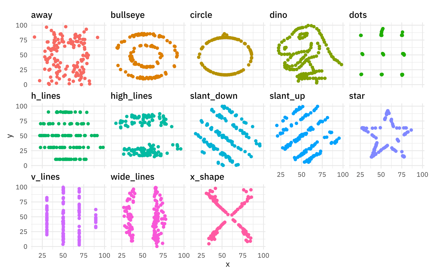
(note that echo = FALSE and eval=TRUE as code chunk options means that the code chunk used to include this image code is run, but not shown)

Source for Image: https://juliasilge.com/blog/datasaurus-multiclass/

34.7 Other languages in code chunks

You can use a number of different open-source languages in addition to R if needed to do your data analysis, including SQL, shell code with Unix Bash, C, C++ via Rcpp, Stan, and D3. Any of these options can be chosen from the Insert Code button dropdown (green +c button).

34.8 Code Chunk Options

When you are working through a data analysis, you usually want to display the code that led to a result. For the final manuscript, you may want to hide the code and just display the results. You can accomplish this with echo=TRUE to display code, and echo=FALSE to hide the code.

Code chunk options should be added to the top of each code chunk, in the chunk header after the name of the code chunk, and separated from the chunk name (and from each other) by commas.

The chunk header (material between the braces) must be written on one line. You must not break the line with a return, or it will not work.

Code Chunk Options
Option	Values	Output
eval	TRUE/FALSE	Whether or not the code is run.
echo	TRUE/FALSE	Show or hide the code
include	TRUE/FALSE	Whether or not the resulting output of a code chunk is displayed in the document. `FALSE` means that the code will run, but will not display results. `include = FALSE` is often used for the setup chunk.
warning	TRUE/FALSE	Whether warnings generated from your code will be displayed in the document.
message	TRUE/FALSE	Whether messages generated from your code will be displayed in the document.
fig.align	default, left, right, center	Where on the page the output figure should align. Text options should be in quotes, like `fig.align = "right"`
fig.width	default = 7	figure width in inches
fig .height	default = 7	figure height in inches
error	TRUE/FALSE	If `TRUE`, will not stop building the document if there is an error in a code chunk.
cache	TRUE/FALSE	If `TRUE`, will store the results and not re-run the chunk. Helpful for long, slow calculations. But watch out for this if your data change and your results do not(!!).

Note that there are many more chunk options which you can use if needed, and these can be found here.

34.9 How It All (Rmarkdown + {knitr} + Pandoc) Works

rmarkdown processing from rstudio.com

Rmarkdown is an R-flavored version of the markdown language. This is a universal, open-source markup language for creating formatted documents from plain text. Markdown documents end with the file extension *.md. An open-source program named pandoc converts *.md documents to output documents like MS Word, PDF, HTML, MS Powerpoint, etc.

When you click the Knit button or run the render() function, R Markdown feeds the .Rmd file to knitr, which executes all of the code chunks and creates a new markdown (.md) document which includes the code and its output.

The markdown file generated by {knitr} is then processed by pandoc which is responsible for creating the finished format.

This may sound complicated, but R Markdown makes it extremely simple by encapsulating all of the above processing into a single render() function (or the Knit button).

34.10 Knitting and Editing (and re-Knitting() Your Rmd document

Find the Knit button at the top of the file, and click it to convert this *.Rmd . It will automagically knit the document first to markdown (to *.md and then from *.md to *.HTML.

Scroll through the document to see what has been created.

Go back to the Rmd document.

Now try the following:

in the YAML header, edit the author to your name
edit the date to the current (or a different) date
edit the output from html_document to word_document
find the glimpse code chunk. After the chunk name glimpse, add a comma, then the option echo=FALSE
Add this same option to a few of of the other code chunks (feel free to use copy-paste, but make sure you don’t end up with duplicate commas, as this will cause errors)
Now click on the Knit button again.

You should get a new version of the document, now in MS Word format, with the code chunks hidden, and a new author and date. The Word document is in a particular default format, but you can change this by specifying a template word file in the YAML header.

34.11 Try Out Other Chunk Options

Try adding different chunk options, including

include = FALSE
eval = FALSE, echo = TRUE
eval=TRUE, echo = FALSE

34.12 The `setup` chunk

The setup chunk is a special code chunk, which is usually the first code chunk at the top of your RMarkdown document. Typically it includes two types of code:

libraries to be loaded
data to be loaded in the background

and often looks something like this:

library(tidyverse)
library(here)
data <- read_csv(here("data/my_data_file.csv"))

(note that for display purposes, I am using the chunk options eval = FALSE, echo = TRUE, while in a real setup chunk, I would use include = FALSE, which runs the code but does not display the code nor the output. I also had to change the chunk name to setup2 because only unique chunk names are allowed).

Scroll to the setup chunk at the top of your Rmd document to see what a working setup chunk looks like.

34.13 Markdown syntax

Markdown is a popular markup language that allows you to add formatting elements to text, including bold, italics, and code formatting.

We make text Bold by surrounding the words with double asterisks. We make text Italic by surrounding the words with single underscores or single asterisks. We make text Bold and Italic by surrounding the words with triple underscores or triple asterisks. We can make text in code-font by surrounding it with single back-ticks.

You can also format level 1 to level 5 headings. These are done by preceding the heading (on its own line) with 1-5 hashtags.

34.14 2nd Header

34.14.1 3rd Header

34.14.1.1 4th level Header

34.14.1.1.1 5th level header

(note that I did not use a level 1 header, which would have forced a new chapter in bookdown). There is only one level 1 header in this chapter - the chapter title.

34.15 Line Breaks and Page Breaks

If you simply hit return in your *.Rmd document, you will see a line break in your text. But this is only a semantic line break, as the knitted document will smush these lines together.

You can create a deliberate line break by adding 2 or more spaces to the end of a line of text. This will work in any output format.

The downside of this is that these line breaks are not visible, until you Knit the document.

Line breaks can be inserted (for HTML output) by
using
html tags
The HTML tag for line breaks is <br>. But these are kind of annoying to type,
and 2 spaces at the end of each line is pretty easy, but less visible when you are looking at the text in the Rmd.

Note that you need a blank line before headers for them to be recognized as headers and formatted properly

34.16 Making Lists

34.16.1 Ordered Lists

You can create an ordered list by preceding items with numbers and period:

First
Second
Third

34.16.2 Un-ordered lists

You can create an un–ordered list with the - + or * keys as your leading bullets.

chickadee
carrot
quartz

34.16.3 Nested Lists

You can create nested lists by tab-indenting with a new symbol, using - for level 1, + for level 2, etc.

Birds
- Hawk
Vegetables
- Carrot
  - Baby
  - Ball
  - Nantes
Minerals
- Gneiss

34.17 The Easy Button - Visual Markdown Editing

While it is helpful to know all of the formatting options for headers, italics, bold, etc. for troubleshooting, it is not as simple as a modern word processor with menu buttons. So RStudio came up with the Visual Markdown Editor.

This can be activated for your RMarkdown document by clicking on a button in the top right of your Rmd document pane. It looks a bit like a compass, or possibly an Angstrom symbol (if you were a chemistry major).

If you toggle this button to on, your Rmarkdown document now has basic word processor functions, including live formatting - What You See Is What You Get (WYSIWIG). A new submenu appears at the top of the document, with buttons to select the heading level (or normal text, or code block), as well as bold, italic, and underline. You can insert lists, tables, block-quotes, links, citations, cross-references within a document, images, horizontal lines, special characters, and math equations. There is a drop-down menu to help you format tables. You can even insert comments into a shared manuscript.

34.17.1 Try inserting a list, a table and a block-quote

In your practice RMarkdown document, from the Rmarkdown Visual Editor View,

Insert a short list of endoscopic procedures, types of dialysis, or interventions done through a catheter
Insert a small 3 column table with columns for ethnicity (Hispanic/Non-Hispanic), retirement status (Retired/Not Retired), and Count
Insert the following as a block quote: “Don’t judge each day by the harvest you reap but by the seeds that you plant.” -Robert Louis Stevenson

34.18 Inline Code

You will often want to insert a result into your text, like a percent reduction in an endpoint, or a p value. Rather than copying and pasting from somewhere else (which are prone to error, or forgetting to update), you can do these calculations right in your text, using inline R code. For example, if you want to say that we evaluated NN COVID PCR tests for this study, you can calculate how many rows in your dataset with R, right in the text.

To do this, you bracket the code with single back-ticks, and start with the letter r immediately after the first back-tick, so that Rmarkdown knows that R code is coming. After the lower-case r, you can insert your code expression, like nrow(covid) to give you the number of rows (observations). Putting this together, this looks like `r nrow(covid)`. When you insert this in the middle of a sentence in your text (inline code), this lets you write sentences in your manuscript like the following, which calculate the actual number in the text (and automatically update when your data changes):
We evaluated 15524 COVID PCR tests in this study.

34.18.1 Try inserting some in-line R code

Try this yourself. Select the correct code to insert the proper results, as illustrated below (note that these would be surrounded by single back-ticks)

The mean cycle threshold in this study was

r covid %>% mean(ct_result, na.rm = TRUE) %>% format(digits = 5) r covid %>% median(ct_result, na.rm = TRUE) %>% format(digits = 7) r covid %>% sd(ct_result, na.rm=TRUE) %>% format(digits =3)

The standard deviation of the cycle threshold in this study was