Chapter 40 Building Data Pipelines with {targets}

This chapter is part of the Reproducibility pathway.
Packages needed for this chapter include {targets}, {tarchetypes}, {gt}, and {gtsummary}.

The {targets} package is a pipeline toolkit for R that allows you to define a sequence of R scripts, functions, and targets, and then run this pipeline in a reproducible and efficient way. The package is designed to help you manage the complexity of your multiple analysis scripts, and to help you keep track of the dependencies between your scripts. The package is particularly useful for large-scale data analysis projects, where you have many scripts that depend on each other, and where you need to keep track of the dependencies between your scripts.

The {targets} package is designed around the idea of a “target”, which is a unit of work that can be run independently of other targets.

A target is usually the output object, which is often a tibble, a formatted table, or a plot.
A function converts an input data object into a target (output data object). Each function is usually derived from a working data script.
Each target depends on the input data and the functions that are used to create it.

Modular Scripts become Functions To Build Pipelines with {targets}

As you build up complex workflows that are sequential, or branching, or unite two different pathways, it helps to have modular scripts that handle distinct functions like

01_read_data
02_cleaning_data
03_wrangling_data
04_making_tables (input is clean_data, output is tables)
05_modeling_data (input is clean_data, output is models)
06_visualizing_data (input is clean_data,output is plots)

Previously, we have set these up as numbered scripts in an RStudio Project, which are meant to be run in order, and have data inputs and object outputs (data tables, models, plots, etc., which can be saved with saveRDS or ggsave)

40.1 What Does {targets} Do?

The {targets} package helps you use these scripts (after being converted to functions), as a pipeline of targets. The {targets} package provides a set of functions for defining targets, running targets, and managing the dependencies between targets. The {targets} package can detect which intermediate steps have already been run and are up-to-date, versus those that have changed scripts or input data, and are out-of-date (and need to be re-run). For small projects, the {targets} package may feel like overkill, but for complex projects, it can greatly help you keep track of the dependencies between your scripts, and help you run your scripts in the correct order in a reproducible and efficient way.

If you have an early step in your data pipeline that uses very large data, is computationally intensive, or simply takes a long while, you do not need to re-run it if {targets} can see that the input data and the data processing functions have not changed. You can be more efficient, and just update the later (downstream) functions and run these.

Let’s start with the example in the {targets} R user manual, using airquality data from base R. A walkthrough can be found in this 4 minute video at
https://vimeo.com/700982360. Take a few minutes to watch the video to get the basic idea of how {targets} works.

The {targets} package is designed to get your computer to help you manage the complexity of your data analysis scripts. In order to get the computer’s help with this, we will be writing code with very specific syntax in very specific files in very specific locations that the computer understands. This makes it pretty easy to make syntax errors and get error messages. If you get an error message, don’t panic! Just read the error message, and try to understand what it is telling you. The {targets}User Manual has a whole chapter on debugging pipelines. The {targets} package is a powerful tool, but it can be a bit finicky. Be patient with yourself as you learn how to use it.

40.2 Air Quality Analysis

Now let’s replicate what Will Landau (author of {targets}, employed at Eli Lilly) just narrated. First, go to your local RStudio and open a File/New Project. Choose a New Directory/New Project, and call it something like ‘airquality’. then Click on the Create Project button. Then, add a folder named ‘R’ to the project in the Files tab in RStudio by clicking on the folder at top left with a green + sign. This is where you will store your functions.

40.2.1 Prepping The Functions.R file

Now, click to enter the R folder you just created in the project, and within the R folder, create a new R script (New File is just to the right of the New Folder button in the Files tab) called ‘functions.R’ and copy the code below (use the copy icon in the top right corner of the code chunk) into this R script. This script will contain all 3 of the functions needed to run this targets pipeline on the airquality data.
Then save the script functions.R.

get_data <- function(file) {
  read_csv(file, col_types = cols()) %>%
    filter(!is.na(Ozone))
}

fit_model <- function(data) {
  lm(Ozone ~ Temp, data) %>%
    coefficients()
}

plot_model <- function(model, data) {
  ggplot(data) +
    geom_point(aes(x = Temp, y = Ozone)) +
    geom_abline(intercept = model[1], slope = model[2])
}

40.2.2 Checking Your Functions

Now, to check that everything is running OK, copy and run (locally in the RStudio Console pane) the code chunk below at the cursor - paste and press Enter/Return. This will load the packages and functions, write the data.csv file, then run each function to get and process the data, then finally draw the plot in your Plots tab.

library(dplyr)
library(ggplot2)
library(tibble)
library(readr)
source("R/functions.R")
airquality |>  write.csv("data.csv", row.names = FALSE)
data <- get_data("data.csv")
model <- fit_model(data)
plot <- plot_model(model, data)
plot

This should all be working, and you should see the resulting plot in the Plots tab. Resulting Plot of Ozone vs. Temp

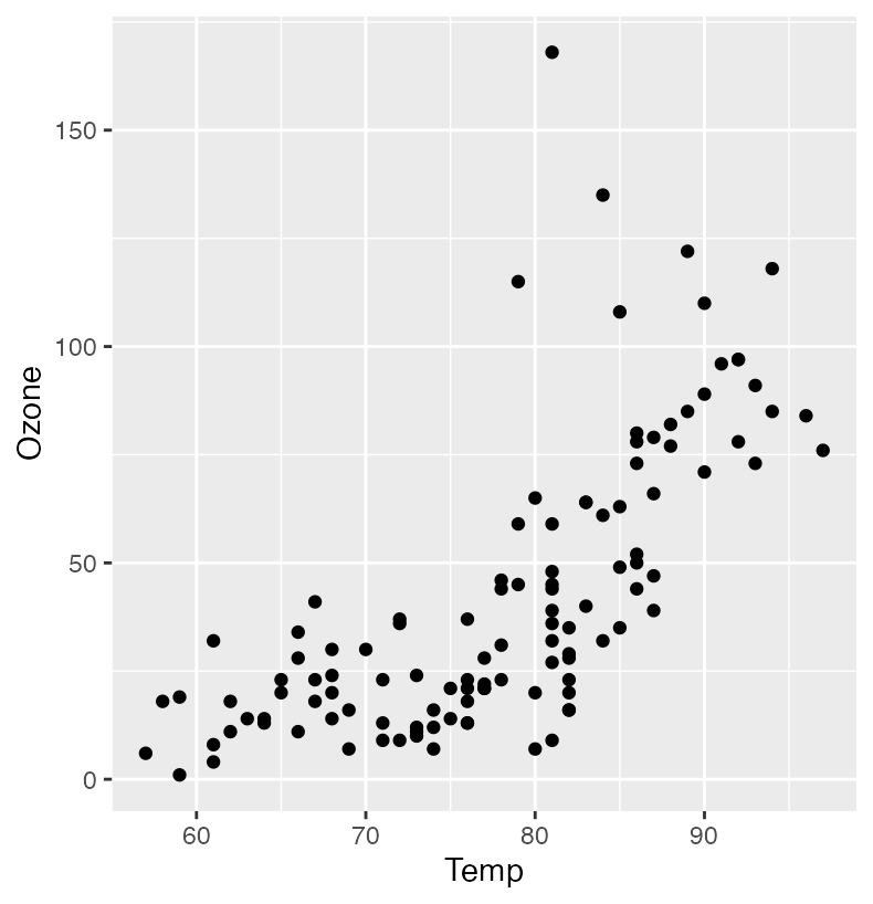
If not, go back and check the functions. This is all good, but it is still functions/scripts, without a {targets} pipeline. But now all the prep work is done, with the initial data file in a new project, and all the coding/processing in a functions script within the R folder. Oftentimes you will have a working script and have to convert it to functions (unless you write your code in functions already) as part of the prep work for a {targets} pipeline. This happens fairly often as you start to scale up projects in size and complexity.

40.2.3 Set Up the Pipeline

Now you are ready to build a pipeline. Run the code chunk below to load {targets} and run the use_targets() function. This will create a new file called ‘_targets.R’ in the root of your project. This script will contain the pipeline code that you will build up in the next steps.

library(targets)
use_targets()

Click on your Files tab and go up one level from the R folder to the root of the project, to confirm that _targets.R file now exists in the root of your project. This file should now be open in your Source pane, and labeled on the tab at the top as _targets.R. This is where you will build up your pipeline.

Within the _targets.R file, scroll down to the tar_option_set() function. This function sets the options for the pipeline, including all of the packages that you will need. For this pipeline, we will need

“tibble”
“readr”
“ggplot2”
“dplyr”

For more complex pipelines, we will need more packages. Take a moment to add the packages to the list (which starts with only “tibble”), Make sure each one is in quotes, and separated by commas (but without a comma at the end). Confirm that there are no syntax errors, and save the file _targets.R.

Now scroll down to the list() function at the end with two tar_targets inside of it.

Our code will need four targets for the pipeline. These target output objects are:

file
data
model
plot

Before we replace the two existing tar_targets, let’s inspect them. Notice that each of the two tar_target() functions currently shown has a first argument that is the target, or output object. The second argument is the function or command that generates the output object (or the datafile if we are just reading in data). The argument for each of these functions is the input object for that function, which is usually generated in the preceding tar_target() function. This pipeline is essentially a chain of input objects transformed to output objects, which become the input objects for the next function in the pipeline.

Looking at our planned airquality pipeline (see code chunk below below),

the first target is file
the second target is data, which is generated by the get_data() function, which uses the file target as input
the third target is model, which is generated by the fit_model() function, which uses the data target as input
the fourth target is plot, which is generated by the plot_model() function, which uses the model and data targets as input

Copy the code chunk below and replace the tar_target() lines (replace everything from the beginning of list( to the closing parenthesis) (everything from line 52 to line 62) with the code below.

list(
  tar_target(file, "data.csv", format = "file"),
  tar_target(data, get_data(file)),
  tar_target(model, fit_model(data)),
  tar_target(plot, plot_model(model, data)
  )
)

Make sure that your list ends with 3 consecutive close parentheses (and a red parenthesis if you are using rainbow parentheses). Check that all the parentheses and commas are correct, with no syntax errors, then save _targets.R again.

40.2.4 Pre-Build Checks

Now we are ready to start building the pipeline. Let’s start with two pre-build checks. First, run tar_manifest() locally in your project in the Console as shown below. This will check the pipeline and show you the status of each target.

tar_manifest(fields = command)

This should generate a table in your console with two columns, showing the name of each target, and the command that generates that target.

tar_manifest Output

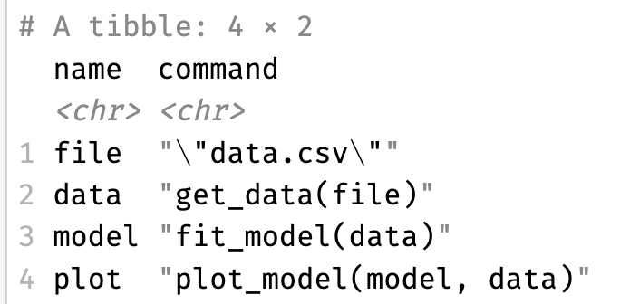
Note that the file target will not have a proper function to generate it, but something that looks like "\"data.csv\"" If you see any errors and don’t get a 4 x 2 table, you will need to fix either the functions.R file and/or _targets.R before proceeding.

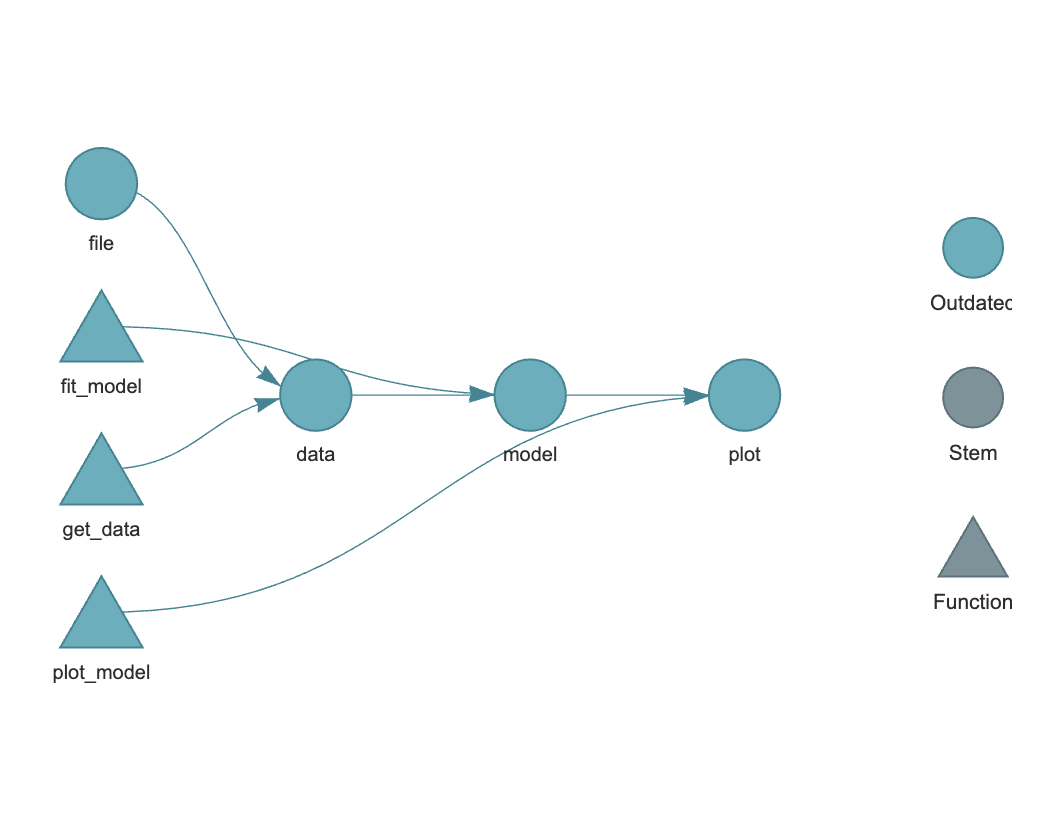
Now we can visualize our pipeline by copying and running the code chunk below in the Console. This will generate a graph of the pipeline, showing the targets and the dependencies between them. The graph should show the four targets, with the file target at the left, and the plot target at the far right. The data target depends on the file target, the model target depends on the data target, and the plot target depends on the model and data targets. There should be a continuous flow from left to right, though it can branch or unite in more complex workflows. As this is a new pipeline, each target will be color coded (a blue-green) as “Outdated”, as each target has not been built yet.

tar_visnetwork()

New Pipeline

### Building the Pipeline

Now that the pre-build checks are good, we are ready to build the pipeline. Run the function below in your local project to build the pipeline.

tar_make()

As this is a new pipeline, it will run (dispatch) every function and create every target anew. The output in the console will tell you when it dispatches each target and when it completes building the target output object, along with how long it takes to run the whole pipeline.

tar_make Output

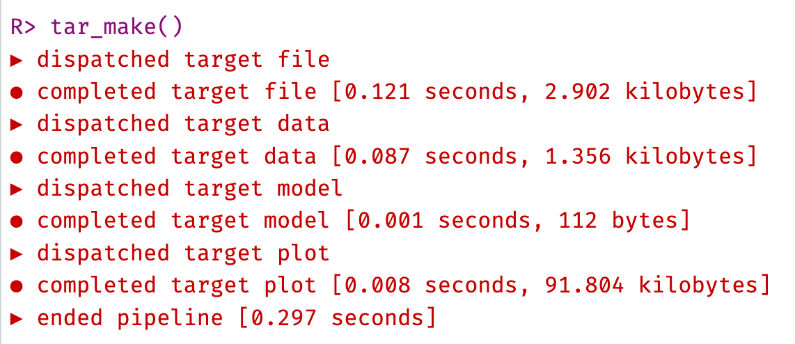
The output objects are also saved to binary files in the _targets/objects/ folder (data, model, and plot). You can check these files (with tar_read(object), rather than clicking on them, as they are binary files and woin’t display like normal R objects) to see the output objects, and this will load these objects into your R session to check them.

For example, to load the plot object, you would run the code below.

tar_read(plot)

Because these target objects are stored and tracked by {targets}, if you re-run tar_make() without any changes to the data or the function code, it will skip all the functions, and complete the pipeline very quickly.

Only if changes are made to the data or code will the pipeline re-run the functions that are affected by the changes. This is a key feature of {targets} that makes it so powerful for efficient, reproducible research.

If you now run tar_visnetwork() again, you will see that the pipeline is now complete, with all the targets built (black). The graph should show all the targets as black, indicating that they are up-to-date.

Run tar_make() again to demonstrate this. You should see that the pipeline runs much faster this time, as nothing needs to be to re-run.

We can demonstrate the tracking ability of {targets} my making minor changes to the data or the functions.

40.2.5 Changing the Pipeline

As an example, let’s change the model to make the model predictor Wind instead of Temp. Copy the code below to replace the fit_model() function in the R/functions.R script. Note that you can also simply type Wind in place of Temp in the function. Save the edited functions.R file. This will change the model output, and the pipeline will have to re-run the model and plot targets, but not the data or file targets.

fit_model <- function(data) {
  lm(Ozone ~ Wind, data = data) |> 
    coefficients() 
}

Now re-run tar_visnetwork() to see the changes in the pipeline. The fit_model function, and the model and plot targets that depend on the model function upstream should now be blue-green, indicating that they are out of date and need to be re-run.

Out of Date Network

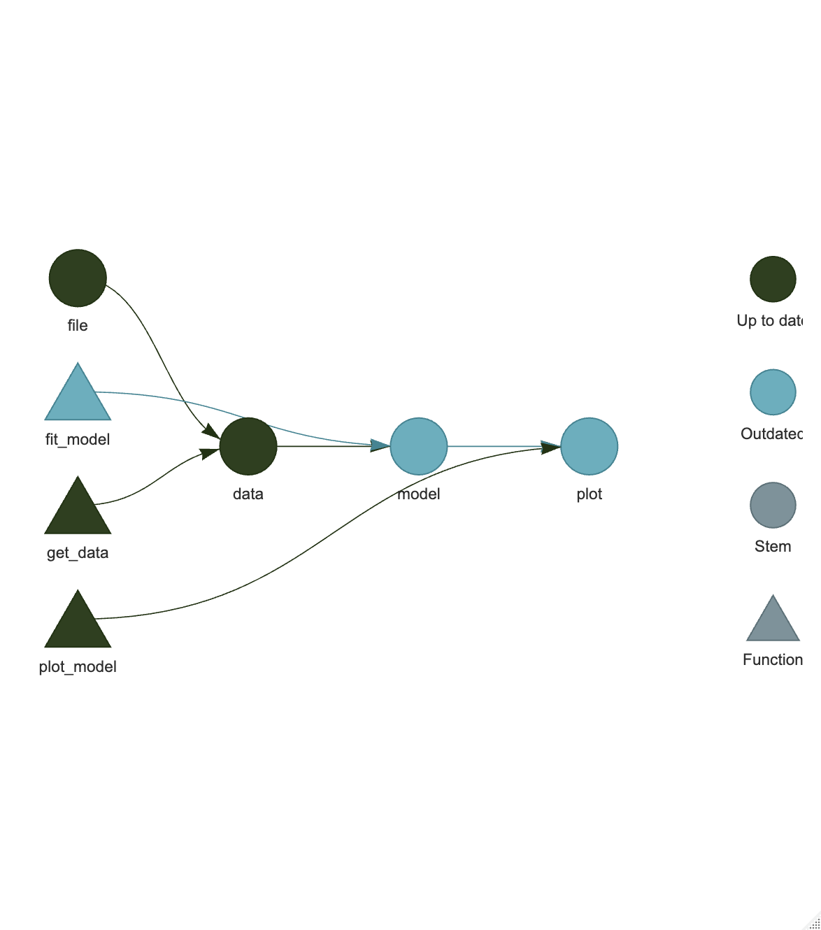
Run tar_make() to re-run the pipeline. You should see that only the model and plot targets are re-run, while the data and file targets are skipped.

Re-running tar_visnetwork again will show that the whole pipeline is now up-to-date (black) again.

This is the power of {targets} - it tracks the dependencies between functions and data, and only re-runs the parts of the pipeline that are affected by changes. This makes it much faster and more efficient than re-running the whole analysis every time you make a change.

40.3 Your Turn - A Tuberculosis Analysis Pipeline

Now it is your turn to convert a set of scripts into functions, then into a targets pipeline. The code block below represents a 5-step analysis of World health Organization (WHO) data on tuberculosis, which are included in the {tidyr} package.

Start by opening a New Project in RStudio, named something like “who_tb_analysis”. Go to the Files tab, then create a new Folder in the project called “R”. Within this folder, create a new File (an RScript) named “functions.R”.

# these functions require: dplyr, gt, gtsummary, ggplot2, tidyr, scales
# 01 read in data

who_data <- tidyr::who

# 02 clean data

who_data %>% pivot_longer(
  cols = new_sp_m014:newrel_f65,
  names_to = c("diagnosis", "gender", "age"),
  names_pattern = "new_?(.*)_(.)(.*)",
  values_to = "count"
  ) |> 
  na.omit() -> 
who_clean


# 03 make table

who_clean |>
  group_by(country) |> 
  summarize(Case_Count = sum(count)) |> 
  slice_max(Case_Count, n= 10) |> 
  gt::gt() |> 
  gt::fmt_number(columns = Case_Count, use_seps = TRUE,decimals = 0)


# 04 Model case counts

model <- lm(count ~ diagnosis + gender + age, data = who_clean )
model |> 
  gtsummary::tbl_regression()


# 05 Plot

who_clean |> 
    group_by( year) |> 
    summarize(sum = sum(count)) |> 
    ggplot(aes(x= year, y = sum)) + 
    geom_point() + 
    labs(title = "WHO Count of TB Cases by Year", y = "Cases", x = "Year") +  
    scale_y_continuous(labels = label_number(scale = 1e-6, suffix = "M")) +
    theme(legend.position = "none")

This is a pretty typical 5-step analysis script. The first step reads in the data, the second step cleans the data, the third step makes a table, the fourth step models the data, and the fifth step plots the data.

Run the script code above in your local session to test out the script, and get a sense of the data. Inspect the inputs and outputs of each step to understand the data and the analysis.

40.3.1 Making new Functions

Now we will convert each of these small scripts into a function, and save these in the functions.R file within the R folder. This can be a big part of the prep work in building a {targets} pipeline. You can try this yourself if you are practicing converting scripts to functions, or you can just click on the button to reveal the solution, and copy the code below into the functions.R file.

# 01 read in data 
read_data <- function(file){ 
  who_data <- read_csv(file,
          col_types = cols())
}

# 02 clean data

clean_data <- function(who_data){ 
  who_data |> 
    pivot_longer(
      cols = new_sp_m014:newrel_f65, 
      names_to = c("diagnosis", "gender", "age"),
      names_pattern = "new_?(.*)_(.)(.*)", values_to = "count" ) |> 
    na.omit() -> 
  who_clean 
}

# 03 make table

make_table <- function(who_clean){
  who_clean |> 
    group_by(country) |> 
    summarize(Case_Count = sum(count)) |>  
    slice_max(Case_Count, n=10) |> 
    gt::gt() |> 
    gt::fmt_number(
      columns = Case_Count, 
      use_seps = TRUE,
      decimals = 0) 
}

# 04 Model case counts

model_cases <- function(who_clean){
  model <- lm(count ~ diagnosis +
gender + age, 
  data = who_clean) 
  model |> 
    gtsummary::tbl_regression()
}

# 05 Plot

plot_data <- function(who_clean){
  plot <- who_clean |> 
    group_by( year) |> 
    summarize(sum = sum(count)) |> 
    ggplot(aes(x= year, y = sum)) +
    geom_point() + 
    labs(title = "WHO Count of TB Cases by Year", 
         y = "Cases", x = "Year") +
    scale_y_continuous(labels = label_number(scale = 1e-6, suffix = "M")) +
    theme(legend.position = "none") 
  return(plot)
}

After copying in the code, now we have to save the functions.R script.

40.3.2 Testing functions

We can test the new functions by running them in the console. Copy and run the lines of code below in the Console to test the functions. Examine the inputs and the output (target) objects (there will be a quiz).

library(tidyverse)
library(scales)
library(gt)
library(gtsummary)
tidyr::who |> write_csv("who_data.csv")
source("R/functions.R") # this loads the functions into the R session
read_data('who_data.csv')
clean_data(who_data)
make_table(who_clean)
model_cases(who_clean)
plot_data(who_clean)

If all of the functions are working, this should have produced:

who_data in the Environment pane
who_clean in the Environment pane
A table of the top 10 countries with the most cases in the Viewer tab
A table from a regression model in the Viewer tab
A plot of the data, with rising cases over time in the Plots tab

TB Cases vs Year Plot

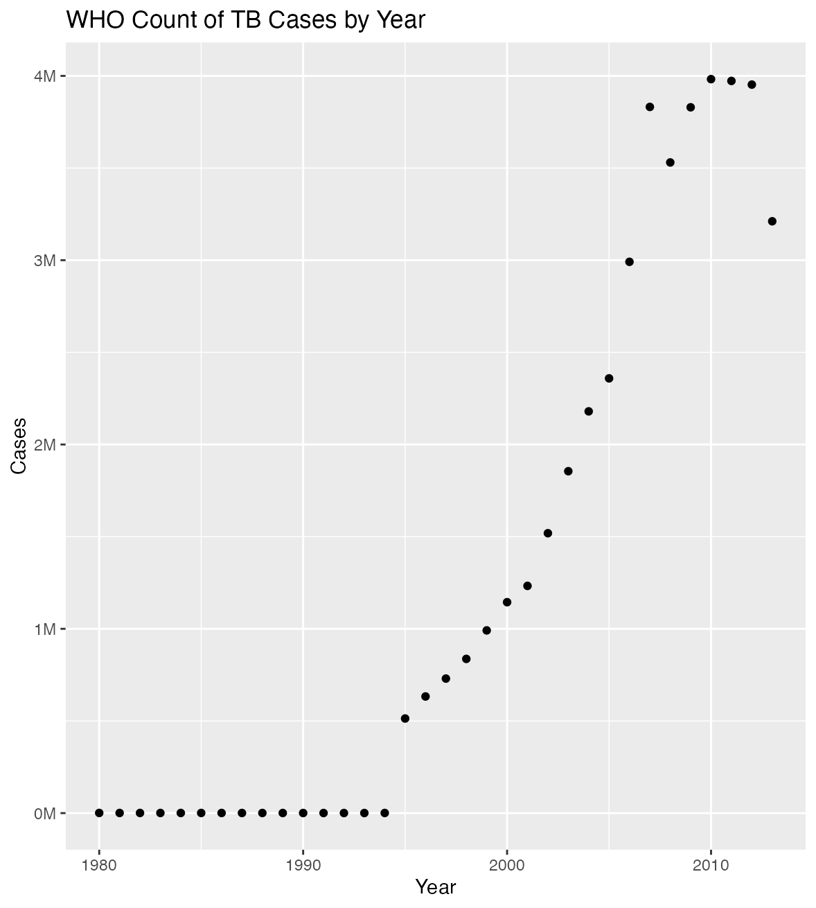
40.3.2.1 Understanding the data (green answers are correct)

What is the name of the raw data object?

What is the name of the cleaned data object?

How is it the clean data object different from the raw data?

How are the age groups in the data defined?

Note the gender codes are obvious, but the diagnosis codes are not - these are sp=sputum, rel = relapse, ep = extra-pulmonary, and new = new cases.
What factors do you expect to be associated with case counts?

40.3.3 Setting Up {targets}

Now that all of the functions are working, to initialize the pipeline, we need to first load {targets}, by running the library(targets) function.

Then we need to run the use_targets() function.

This will create a _targets.R file in the R folder. We can then edit this to start building the pipeline. We need to make sure we have added all the packages, and identified all the targets.

40.4 Editing the `_targets.R` File

We will add the required packages to the targets pipeline in the _targets.R file. Scroll down to tar_option_set and find the list of packages. Add the following 7 packages to the list:

tidyr
readr
ggplot2
dplyr
gt
gtsummary
scales.

Be sure that these are all in quotes, within the c() parentheses and appropriate commas without syntax errors. Save the _targets.R file.

Now scroll down to the list of tar_targets. For this pipeline, {targets} will have 6 targets to track.

file
who_data
who_clean
make_table
model_cases
plot_data

Replace the existing targets with these targets by replacing the entire list, using the code chunk below. Now save the _targets.R file.

list(
    tar_target(file, "who_data.csv", format = "file"),
    tar_target(who_data, read_data(file)),
    tar_target(who_clean, clean_data(who_data)),
    tar_target(table, make_table(who_clean)),
    tar_target(model, model_cases(who_clean)),
    tar_target(plot, plot_data(who_clean))
)

Now we have the infrastructure installed.

We can now do our two pipeline pre-checks:

tar_manifest() - should produce a 6 x 2 tibble of targets.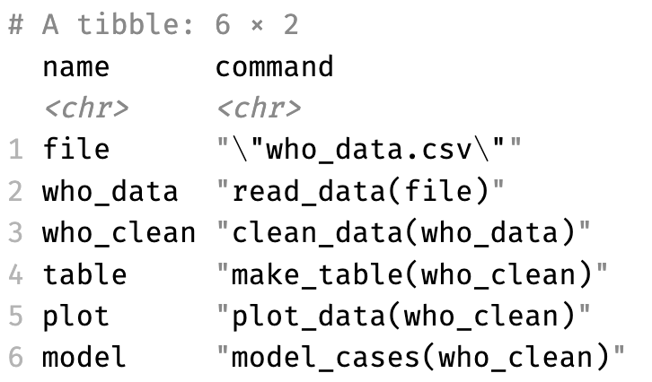

- tar_visnetwork() - should make a completely blue-green (outdated) diagram of the pipeline. tar_manifest Output

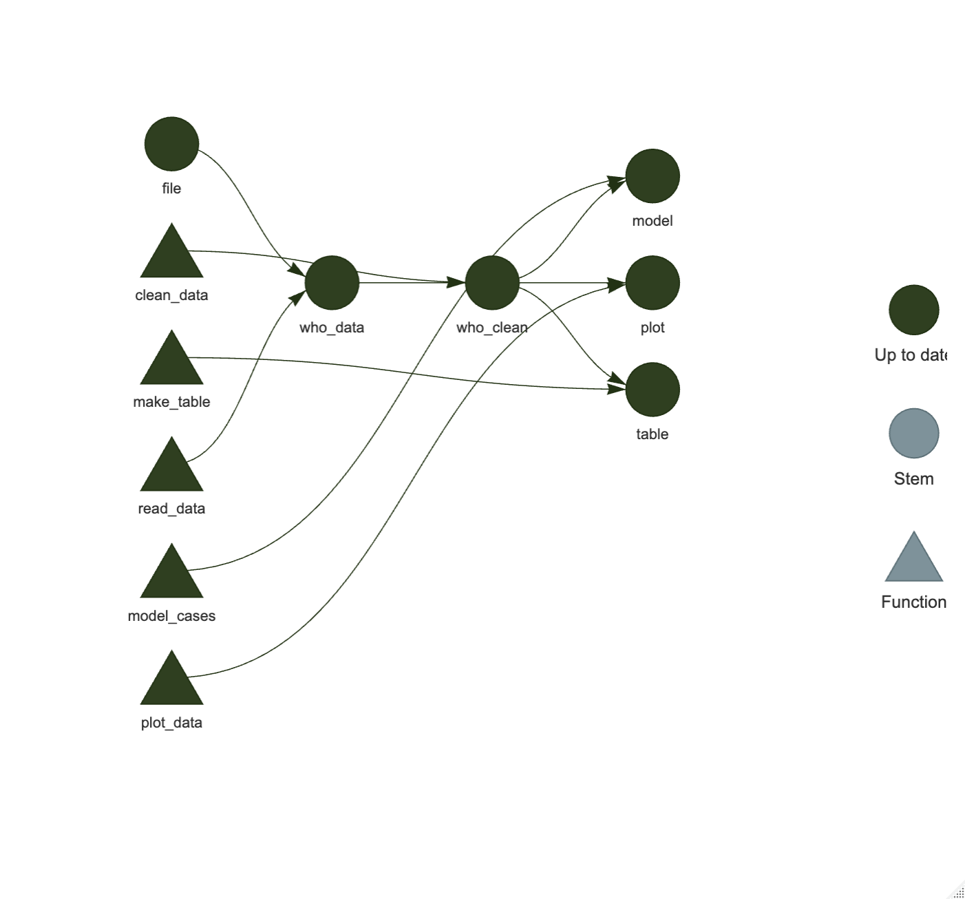
Make sure each of these runs without errors. If not, re-check the steps to create these two files for the pipeline.

functions.R
_targets.R

40.4.1 Running the Pipeline

Once these are running without errors, we can run the pipeline with tar_make().

tar_make Output

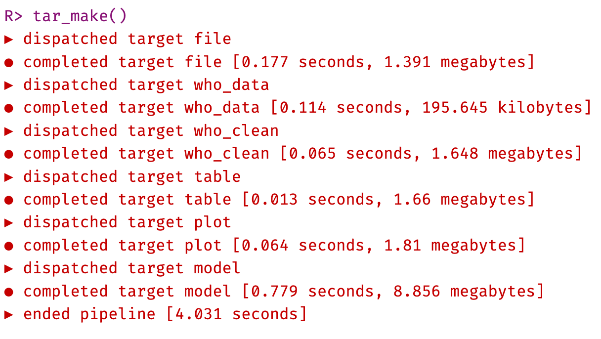
This will run the pipeline and create the outputs in the _targets/objects folder. Check that these are present, and view each target object in the objects folder with tar_read().

Check the output of tar_visnetwork() to see that the pipeline structure is now completely up to date (black targets).

40.4.2 Modificatons to the Pipeline

Now modify the make_table function so that countries with over 1 million cases (scary bad, in need of WHO intervention) are in red text. Use the code below (adding conditional formatting) to edit the make_table() function in the functions.R file in the R folder of the Project. Look carefully at the tab_style() function below to see how the conditional formatting is applied. Make sure that your function ends with 2 close parenthesesm, followed by a closing curly-brace.

who_clean |>
  group_by(country) |> 
  summarize(Case_Count = sum(count)) |> 
  slice_max(Case_Count, n= 10) |> 
  gt::gt() |> 
  gt::fmt_number(columns = Case_Count, use_seps = TRUE,decimals = 0) |> 
  tab_style(
    style = list(
      cell_text(color = "red")
      ),
    locations = cells_body(
      columns = Case_Count,
      rows = Case_Count > 1000000
    ))

Save your modified functions.R file. Run tar_visnetwork() to check on what is now out of date in the pipeline, and then run tar_make() to update the pipeline with the new function. Note that some targets are skipped.

Check out the appearance of the newly-modified table with tar_read(table).

new table

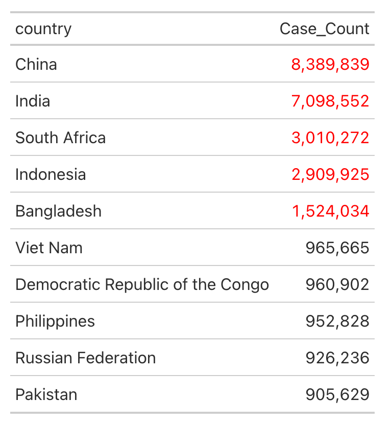
Confirm that the pipeline is now up to date with tar_visnetwork().

40.4.3 Modify the Plot

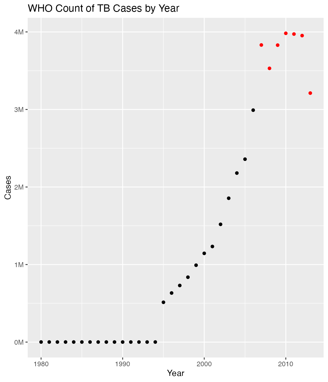
Now modify the plot to make years with greater than 3 million cases of TB have points that are colored red. Use the code below to edit the plot_data() function in the functions.R file in the R folder of the Project.

Look carefully at the aes(color) and scale_color_manual() functions to see how the conditional formatting is applied to point color. Make sure that your modified function has no syntax errors, end with the right number of parentheses, and a final closing curly-brace.

plot_data <- function(who_clean){
  who_clean |> 
    group_by( year) |> 
    summarize(sum = sum(count)) |> 
    ggplot(aes(x= year, y = sum, color = sum > 3000000)) +
    geom_point() + 
    labs(title = "WHO Count of TB Cases by Year", 
         y = "Cases", x = "Year") +
    scale_y_continuous(labels = label_number(scale = 1e-6, suffix = "M")) +
    theme(legend.position = "none") +
    scale_color_manual(values = c("TRUE" = "red", "FALSE" = "black"))
  return(plot)
}

new TB plot with conditional color

Run tar_visnetwork() to check on what is now out of date in the pipeline, and then run tar_make() to update the pipeline with the new function.

Check out the appearance of the newly-modified plot with tar_read(plot)

40.5 Next Steps

You now understand the basics of the {targets} package, and how to build a pipeline. You can now use this approach to build much larger and more complex pipelines for your data analysis projects.

Read much more about the {targets} package in the Targets Package User Manual here.

Challenge yourself:
Convert one of your existing script-based pipelines to a function-based pipeline using {targets}.

Chapter 40 Building Data Pipelines with {targets}

40.1 What Does {targets} Do?

40.2 Air Quality Analysis

40.2.1 Prepping The Functions.R file

40.2.2 Checking Your Functions

40.2.3 Set Up the Pipeline

40.2.4 Pre-Build Checks

40.2.5 Changing the Pipeline

40.3 Your Turn - A Tuberculosis Analysis Pipeline

40.3.1 Making new Functions

40.3.2 Testing functions

40.3.2.1 Understanding the data (green answers are correct)

40.3.3 Setting Up {targets}

40.4 Editing the _targets.R File

40.4.1 Running the Pipeline

40.4.2 Modificatons to the Pipeline

40.4.3 Modify the Plot

40.5 Next Steps

40.4 Editing the `_targets.R` File