Chapter 20 Simple example of a t-test

mtcars %>% 
  filter(cyl ==4 | cyl ==6) %>% 
  mutate(cyl_f = as.factor(cyl)) %>% 
  t.test(mpg ~ cyl_f, data = .)


    Welch Two Sample t-test

data:  mpg by cyl_f
t = 4.7191, df = 12.956, p-value = 0.0004048
alternative hypothesis: true difference in means between group 4 and group 6 is not equal to 0
95 percent confidence interval:
  3.751376 10.090182
sample estimates:
mean in group 4 mean in group 6 
       26.66364        19.74286

20.1 Common Problem

Comparing two groups
- Mean or median vs. expected
- Two arms of study - independent
- Pre and post / spouse and partner / left vs right arm – paired groups
Are the means significantly different?
Or the medians (if not normally distributed)?

20.1.1 How Skewed is Too Skewed?

Formal test of normality = Shapiro-Wilk test
Use base data set called ToothGrowth

library(tidyverse)
library(medicaldata)
data <- cytomegalovirus
head(data)

##   ID age sex race                    diagnosis
## 1  1  61   1    0       acute myeloid leukemia
## 2  2  62   1    1         non-Hodgkin lymphoma
## 3  3  63   0    1         non-Hodgkin lymphoma
## 4  4  33   0    1             Hodgkin lymphoma
## 5  5  54   0    1 acute lymphoblastic leukemia
## 6  6  55   1    1                myelofibrosis
##   diagnosis.type time.to.transplant prior.radiation
## 1              1               5.16               0
## 2              0              79.05               1
## 3              0              35.58               0
## 4              0              33.02               1
## 5              0              11.40               0
## 6              1               2.43               0
##   prior.chemo prior.transplant recipient.cmv donor.cmv
## 1           2                0             1         0
## 2           3                0             0         0
## 3           4                0             1         1
## 4           4                0             1         0
## 5           5                0             1         1
## 6           0                0             1         1
##   donor.sex TNC.dose CD34.dose CD3.dose CD8.dose TBI.dose
## 1         0    18.31      2.29     3.21     0.95      200
## 2         1     4.26      2.04       NA       NA      200
## 3         0     8.09      6.97     2.19     0.59      200
## 4         1    21.02      6.09     4.87     2.32      200
## 5         0    14.70      2.36     6.55     2.40      400
## 6         1     4.29      6.91     2.53     0.86      200
##   C1/C2 aKIRs cmv time.to.cmv agvhd time.to.agvhd cgvhd
## 1     0     1   1        3.91     1          3.55     0
## 2     1     5   0       65.12     0         65.12     0
## 3     0     3   0        3.75     0          3.75     0
## 4     0     2   0       48.49     1         28.55     1
## 5     0     6   0        4.37     1          2.79     0
## 6     0     2   1        4.53     1          3.88     0
##   time.to.cgvhd
## 1          6.28
## 2         65.12
## 3          3.75
## 4         10.45
## 5          4.37
## 6          6.87

20.1.2 Visualize the Distribution of data variables in ggplot

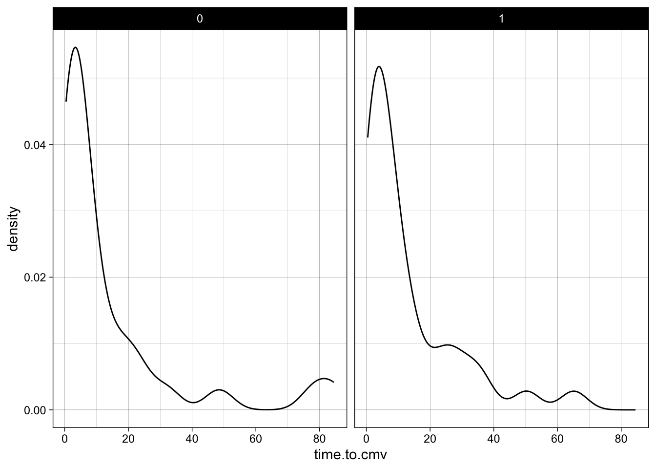
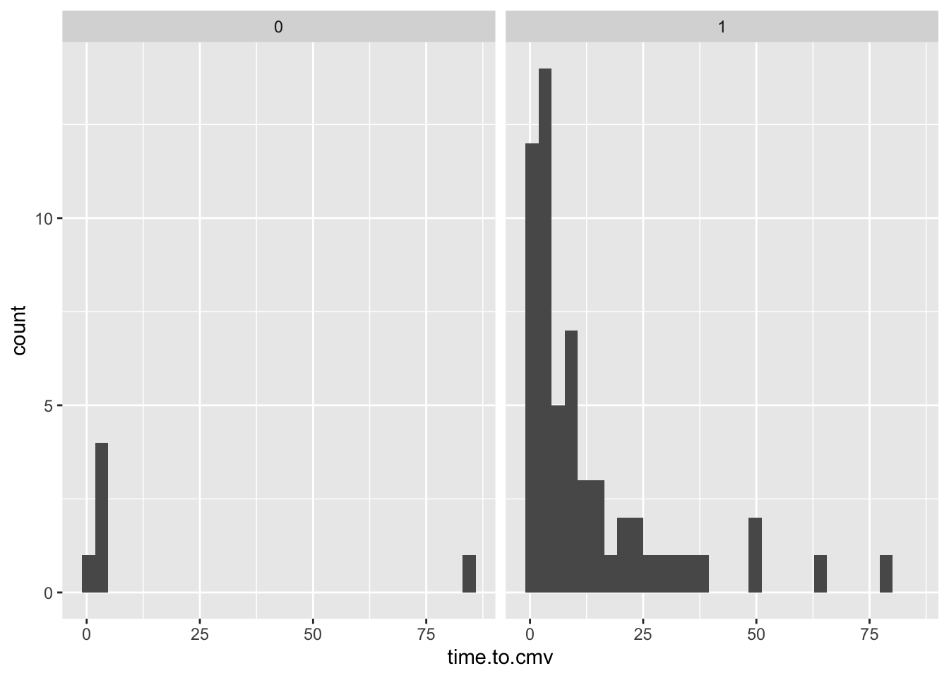
Use geom_histogram or geom_density (pick one or the other)
look at the distribution of CD3.dose or time.to.cmv
Bonus points: facet by sex or race or donor.cmv
Your turn to try it

library(tidyverse)
library(medicaldata)

data %>% 
ggplot(mapping = aes(time.to.cmv)) +
  geom_density() +
  facet_wrap(~sex) +
  theme_linedraw()

library(tidyverse)
library(medicaldata)
 
data %>% 
ggplot(mapping = aes(time.to.cmv)) +
  geom_histogram() +
  facet_wrap(~race)

20.1.3 Visualize the Distribution of data$len in ggplot

The OJ group is left skewed
May be problematic for using means
formally test with Shapiro-Wilk

library(tidyverse)
library(medicaldata)

data$time.to.cmv %>% 
shapiro.test()

## 
##  Shapiro-Wilk normality test
## 
## data:  .
## W = 0.68261, p-value = 0.0000000001762

20.1.4 Results of Shapiro-Wilk

p-value = 0.1091
p not < 0.05
Acceptably close to normal
OK to compare means rather than medians
can use t test rather than wilcoxon test
- if p is < 0.05, use wilcoxon test
- also known as Mann-Whitney test
- a rank-based (non-parametric) test

20.1.5 Try it yourself

use df <- msleep

library(tidyverse)
library(medicaldata)

df <- msleep 
head(df$sleep_total)

## [1] 12.1 17.0 14.4 14.9  4.0 14.4

test the normality of total sleep hours in mammals

20.1.6 Mammal sleep hours

library(tidyverse)
library(medicaldata)

shapiro.test(df$sleep_total)

## 
##  Shapiro-Wilk normality test
## 
## data:  df$sleep_total
## W = 0.97973, p-value = 0.2143

meets criteria - acceptable to consider normally distributed
now consider - is the mean roughly 8 hours of sleep per day?

20.2 One Sample T test

univariate test
- Ho: mean is 8 hours
- Ha: mean is not 8 hours
can use t test because shapiro.test is NS

20.2.1 How to do One Sample T test

library(tidyverse)
library(medicaldata)

t.test(df$sleep_total, alternative = "two.sided",
       mu = 8)

Try it out, see if you can interpret results

20.2.2 Interpreting the One Sample T test

## 
##  One Sample t-test
## 
## data:  df$sleep_total
## t = 4.9822, df = 82, p-value = 0.000003437
## alternative hypothesis: true mean is not equal to 8
## 95 percent confidence interval:
##   9.461972 11.405497
## sample estimates:
## mean of x 
##  10.43373

p is highly significant
- can reject the null, accept alternative
- sample mean 10.43, CI 9.46-11.41

20.2.3 What are the arguments of the t.test function?

x = vector of continuous numerical data
y= NULL - optional 2nd vector of continuous numerical data
alternative = c(“two.sided”, “less”, “greater”),
mu = 0
paired = FALSE
var.equal = FALSE
conf.level = 0.95
documentation

20.3 Insert flipbook for ttest here

Below is a flipbook.
It illustrates a bit of how to do a t-test.
click on it and you can use the arrow keys to proceed forward and back through the slides, as you add lines of code and more results occur.

Let’s start with a flipbook slide show. When the title slide appears, you can step through each line of the code to see what it does. The right/left and/or up/down arrows will let you move forward and backward in the code.

You can use the arrow keys to go through it one step at a time (forward or backward, depending on which arrow key you use), to see what each line of code actually does.

Give it a try below. See if you can figure out what each line of code is doing.

20.3.1 Flipbook Time!

This is t-testing in action.

20.4 Fine, but what about 2 groups?

consider df$vore

library(tidyverse)
library(medicaldata)
prostate <- medicaldata::blood_storage
tabyl(prostate$AA)

##  prostate$AA   n   percent
##            0 261 0.8259494
##            1  55 0.1740506

hypothesis - herbivores need more time to get food, sleep less than carnivores
how to test this?
- normal, so can use t test for 2 groups

20.4.1 Setting up 2 group t test

formula interface: outcome ~ groupvar

library(tidyverse)
library(medicaldata)

df %>% 
  filter(vore %in% c("herbi", "carni")) %>% 
  t.test(formula = sleep_total ~ vore, data = .)

Try it yourself
What do the results mean?

20.4.2 Results of the 2 group t test

## 
##  Welch Two Sample t-test
## 
## data:  sleep_total by vore
## t = 0.63232, df = 39.31, p-value = 0.5308
## alternative hypothesis: true difference in means between group carni and group herbi is not equal to 0
## 95 percent confidence interval:
##  -1.911365  3.650509
## sample estimates:
## mean in group carni mean in group herbi 
##           10.378947            9.509375

20.4.3 Interpreting the 2 group t test

Welch t-test (not Student)
- Welch does NOT assume equal variances in each group
p value NS
accept null hypothesis
- Ho: means of groups roughly equal
- Ha: means are different
- 95% CI crosses 0
Carnivores sleep a little more, but not a lot

20.4.4 2 group t test with wide data

You want to compare column A with column B (data are not tidy)
Do mammals spend more time awake than asleep?

library(tidyverse)
library(medicaldata)

t.test(x = df$sleep_total, y = df$awake, data = msleep)

20.4.5 Results of 2 group t test with wide data

library(tidyverse)
library(medicaldata)

t.test(x = df$sleep_total, y = df$awake, data = msleep)

## 
##  Welch Two Sample t-test
## 
## data:  df$sleep_total and df$awake
## t = -4.5353, df = 164, p-value = 0.00001106
## alternative hypothesis: true difference in means is not equal to 0
## 95 percent confidence interval:
##  -4.498066 -1.769404
## sample estimates:
## mean of x mean of y 
##  10.43373  13.56747

20.5 3 Assumptions of Student’s t test

Sample is normally distributed (test with Shapiro)
Variances are homogeneous (homoskedasticity) (test with Levene)
Observations are independent

not paired like left vs. right colon
not paired like spouse and partner
not paired like measurements pre and post Rx

20.5.1 Testing Assumptions of Student’s t test

Normality - test with Shapiro
- If not normal, Wilcoxon > t test
Equal Variances - test with Levene
- If not equal, Welch t > Student’s t
Observations are independent
- Think about data collection
- are some observations correlated with some others?
- If correlated, use paired t test

20.6 Getting results out of t.test

Use the tidy function from the broom package
Do carnivores have bigger brains than insectivores?

library(tidyverse)
library(medicaldata)
library(broom)

df %>% 
  filter(vore %in% c("carni", "insecti")) %>% 
t.test(formula = brainwt ~ vore, data = .) %>% 
  tidy() ->
result
result

20.6.1 Getting results out of t.test

## # A tibble: 1 × 10
##   estimate estimate1 estimate2 statistic p.value parameter
##      <dbl>     <dbl>     <dbl>     <dbl>   <dbl>     <dbl>
## 1   0.0577    0.0793    0.0216      1.20   0.253        12
## # ℹ 4 more variables: conf.low <dbl>, conf.high <dbl>,
## #   method <chr>, alternative <chr>

20.7 Reporting the results from t.test using inline code

use backticks before and after, start with r
- i.e. My result is [backtick]r code here[backtick].
The mean brain weight for carnivores was 0.0792556
The mean brain weight for herbivores was 0.02155
- The difference was 0.0577056
The t statistic for this Two Sample t-test was 1.1995501
The p value was 0.2534631
- The confidence interval was from -0.05 to 0.16

20.7.1 For Next Time

Skewness and Kurtosis
Review Normality
- When to use Wilcoxon
Levene test for equal variances
- When to use Welch t vs. Student’s t
Paired t and Wilcoxon tests