7 Wind

7.1 Motivation

Wind is a very important factor of Earth climate. It is the main phenomenon that transport matter and energy between different location on the globe and layers of the atmosphere. Wind properties, like speed and direction, can vary a lot. For example, it can be ranged from a smooth breeze to a storm or a hurricane. In case of hurricanes, it is normally a devastating disturbance that can reach a very destructive power on earth ecosystems. Moreover wind is also the main way many plant disperse seeds and pollen. Animals as well use wind for movement. Finally winds also shapes the earth surface trough erosion of rocks and sediments movement.

7.2 Background

Wind can be represented as a vector in 3 dimensions, two on the horizontal plan (\(u\) and \(v\)) and one vertical (\(w\)). However, the vertical wind component is small and its means is by definition 0 so it is often not included in wind measurements. In this scenario the wind is commonly expressed in angular format, with the total intensity on the horizontal plan and the direction.

The fact that the wind is a 3d vector and has this two formats leads to complexities in handling wind data. In particular the direction cannot be averaged directly, as it’s a circular variable, but can needs to be transformed to the vector components, averaged and then transformed back to an angle.

The average of the wind speed can lead to problems as there two different, but both correct ways to do it (Grange 2014). The first one is doing the averages of the vector components, the second one is doing the average of the absolute values of the wind speed. The first method will always result in smaller values, as wind from opposite direction can be averaged to zero. In the following protocol the average of the absolute values will be used.

Lastly, the are several conflicting ways to define the wind direction, when using vectors the direction is the where the wind is going, but in weather forecast the wind direction is where the wind is coming from. Finally also the definition of the orientation of the u and v components can change between different instruments and software.

If there is a neutrally stratified atmosphere, which means there are no important turbulent fluxes, the wind speed above the canopy can be modeled. Due to the friction with the surface the closest the wind is to the canopy the lower the speed, reaching zero at the boundary. The wind profile can be estimated with the following formula:

\[u(z) = \frac{u_*}{k} ln(\frac{z-d}{z_0})\] where:

• \(z\) in \((m)\) is the height

• \(u(z)\) in \((m/s)\) is the speed of the wind at height z

• \(u_*\) in \((m/s)\) is the friction velocity. This is independent from the height and indicates the mechanical turbulence. It can be calculated using this equation \(\sqrt{\frac{1}{\rho} u^\prime w^\prime}\)

• \(k\) is the Von Karman constant (0.4)

• \(z_0\) in \((m)\) is the height where the wind speed is theoretically zero. It can be estimated as 0.1 the canopy height.

• \(d\) in \((m)\) is the displacement height, which accounts for the shift of the wind profile to the presence of a canopy. It can be estimated as \(2/3\) of the canopy height.

7.3 Sensors and measuring principle

There are many types of instruments used for measuring wind speed. Here some of them will be described.

Cup Anemometer : it consists of a set of three cups, crossing a vertical basement stick. This cross shape allows to measure the horizontal wind velocity at a specific height. The wind speed is derived from number of cycles/time or turning velocity. For measuring the wind direction, a wind vane is used. It points to the direction where the wind is coming. This is through a potentiometer to detect the right direction.

Propeller anemometer : the way this this instrument works is very similar to the cup anemometer. It points to the mean wind direction at that moment. With the use of three propeller anemometer pointing different direction, three dimensional wind can be measured.

Ultrasonic anemometer thermometer : This uses the speed of sound to measure the wind. Normally, it will be displayed in three directions to measured all directions and get a more accurate measurement value. One of the advantages of using the ultrasonic anemometer is the small fluctuations detected on the measures. The speed of sounds depends on temperature and air humidity. Thus, the following equations allow the calculation of speed of sound and the temperature at high frequencies;

\[C_l=\frac{D}{2}(\frac{1}{time_A-A}+\frac{1}{time_B-A})\] \[C_l=\sqrt{K_a*R_a*T_{av}}\]

Where:

• \(K_a = 1.4\)
• \(R_a = 287.05 J/Kg*K\)
• \(T_{av} = T(1+0.513*q)\)

Hot wire anemometer : When a current flow is introduce within a wire, there is a release of heat. Then, the air flow goes throguh the wire and cools down removing the released energy. It can be apply in two different ways;

At a constant current, the change of temperature is measure with a thin thermocouple. This can be hard at a high speed wind.

At a constant temperature, with a temperature change the current is regulated, such that the temperature is held constant and thus, with a high wind there will be a high current as well.

Each type of anemometer has its more limitations. For example the starting speed of cup and propeller anemometer is that it starts to rotate when speed is 0.5 m/s. When wind flow stops, but the cup anemometer keeps rotating a bit longer until it fully stops. In case of low wind speed, sonic anemometer are the best instruments to use but in case or rain, it cannot do measurements instead.

During installation the anemometers there are some tips to take into account. Better to set them far above ground, this way the roughness of the lower layer above soil’s surface will not be affecting the measures. The same with any other object around in the area. In case of sonic anemometer, is important to protect it against birds or any type of insect that make small variation when measuring.

7.4 Analysis

library(tidyverse)
library(lubridate)
library(clifro) # for windrose
library(patchwork)
library(ggthemes)
theme_set(theme_bw()) # ggplot theme

wind <- read_csv(here::here("Data_lectures/7_Wind/Winddata_Botanical_garden.csv")) %>% 
  drop_na() %>% 
  rename(WS_0.5m = WS_05m, wd=WD_deg)

deg2rad <- function(deg) deg * pi / 180
rad2deg <- function(rad) rad * 180 / pi

# calculates the wind angular average over the provide input.
# intend to be used together with group_by and summarize
wind_dir_average <- function(wd){
  dir <- deg2rad(wd)
  # calc the vector components and then make the mean
  u <- cos(dir) %>% mean
  v <- sin(dir) %>% mean
  # convert back to a direction. Note atan2 uses y,x
  avg_dir <- atan2(v, u)
  # need to convert in 0 - 360 range
  avg_dir <- avg_dir %% (2*pi)
  return(rad2deg(avg_dir))
}

# wind gathered
wind_g <- wind %>% 
  gather("height", "windspeed", WS_0.5m, WS_1m, WS_2m, WS_5m, WS_10m) %>% 
  # converts the height into a numeric value
  mutate(height = as.numeric(gsub(".*?([0-9]+).*", "\\1", height))) 

wind_1d<- wind %>%
  mutate(Date = floor_date(Date, unit = "1 day")) %>% 
  group_by(Date) %>%
  summarise(across(c(-wd), mean), wd = wind_dir_average(wd))

wind_g_1d <- wind_1d %>% 
  gather("height", "windspeed", WS_0.5m, WS_1m, WS_2m, WS_5m, WS_10m) %>% 
  # converts the height into a numeric value
  mutate(height = as.numeric(gsub(".*?([0-9\\.]+).*", "\\1", height))) 

7.4.1 Wind averages

The wind speed and direction have been averaged at 1 hour. Vectorial average has been used for wind direction. In figure 7.1 the average direction is compared with the original data. Between the 15th and the 16th of January there are some data points with a wind direction close to 0 °N, but the average is around 350 °N.

wind_1h <- wind %>%
  group_by(round_date(Date, unit = "1 hour")) %>%
  summarise(across(-wd, mean), wd = wind_dir_average(wd))

wind %>%
  filter(between(Date, as_datetime("2021-01-15") , as_datetime("2021-01-17"))) %>%
ggplot()+
  geom_point(aes(Date, wd, colour="10 mins"), size=.8) +
  geom_line(aes(Date, wd, colour="1 hour"),
            data=filter(wind_1h, between(Date, as_datetime("2021-01-15"),
                                               as_datetime("2021-01-17")))) +
  labs(y="Wind direction [°N]", colour="Frequency") +
  scale_y_continuous(breaks = c(0, 90, 180, 270, 360),
                     labels = c('N (0°)', 'E (90°)', 'S(180°)',
                                'W(270°)', 'N (360°)'), limits = c(-10, 370)) +
  scale_color_colorblind()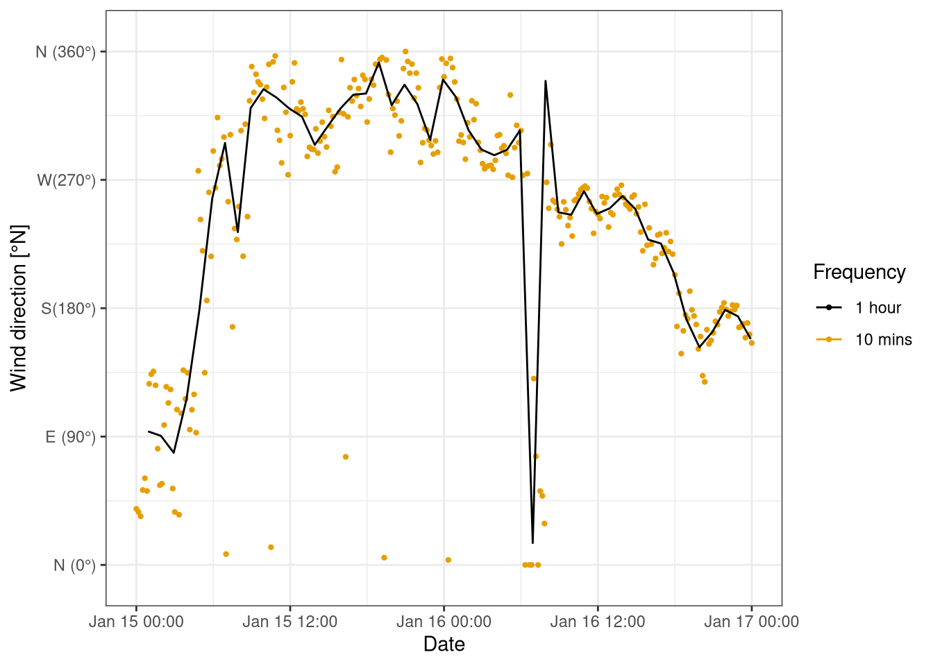

Figure 7.1: Comparison of wind direction original data (10 mins) and hourly average. Data from botanical garden 15th-17th January 2021.

7.4.2 Wind speed and height

As it is possible to appreciate in Figure 7.2 , wind speed gets faster at 10m height. This makes sense when having in mind the vertical wind profile graph that increases with height. The pattern is also consistent across different seasons.

Wind speed depends on height, increasing with height following a logarithmic profile (Figure 7.3). The plot was made using daily averages instead of high frequency data, to reduce the variation in the dataset.

(wind_g_1d %>%
  #just one month otherwise the plot is too compressed
  filter(between(Date, as_datetime("2020-01-15") , as_datetime("2020-02-15") )) %>% 
  mutate(height = fct_reorder(as_factor(height), sort(height, decreasing = T))) %>% 
  ggplot(aes(Date, windspeed, col=height))+
  geom_line() +
  scale_color_colorblind() +
  labs(y="Windspeed [m/s]", colour="Height [m]", title="(a) Winter month")) /
(wind_g_1d %>%
  #just one month otherwise the plot is too compressed
  filter(between(Date, as_datetime("2020-06-15") , as_datetime("2020-07-15") )) %>% 
  mutate(height = fct_reorder(as_factor(height), sort(height, decreasing = T))) %>% 
  ggplot(aes(Date, windspeed, col=height))+
  geom_line() +
  scale_color_colorblind() +
  labs(y="Windspeed [m/s]", colour="Height [m]", title="(b) Summer month")) +
plot_layout(guide="collect")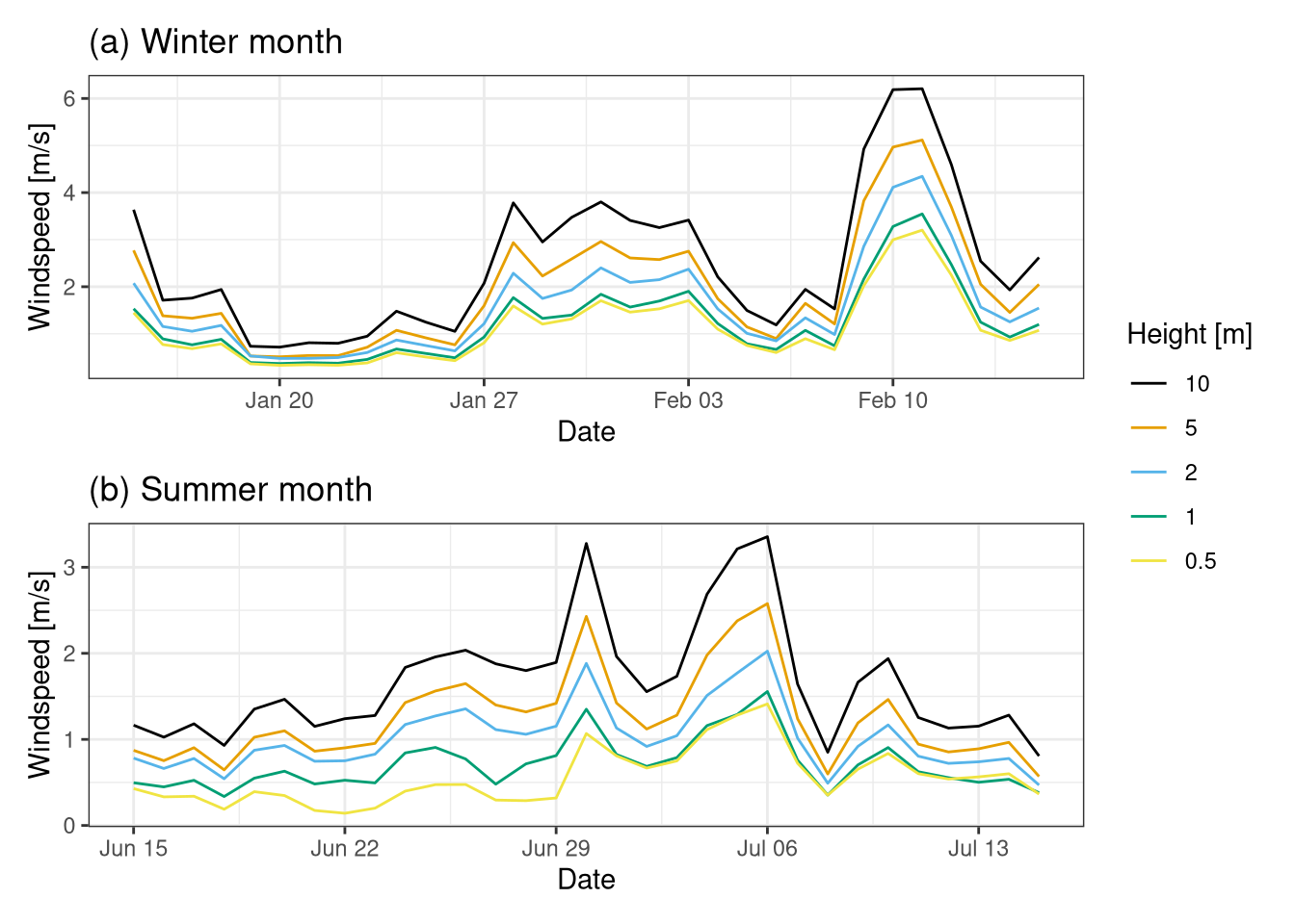

Figure 7.2: Time series of wind speed at different heigth. (a) is a summer month (15th Jan 2020 - 15th Feb 2020). (b) is a winter month(15th Jun 2020 - 15th Jul 2020). Data from botanical garden.

wind_prof <- wind_g_1d %>% 
  group_by(height) %>% 
  summarize(windspeed=mean(windspeed))
#### fit logarithmic wind profile to data and estimate the parameters u*, z0 and d
# initial values
u_star_start <- 0.1
d_start <- 0.3
z0_start <- 0.05

log_prof_model <- nls(windspeed ~u_star/0.4*(log((height - d)) - log(z0)), 
                 start = list(u_star=u_star_start,              
                              d=d_start,              
                              z0=z0_start),                     
                 na.action = na.exclude, data=wind_prof)
wind_prof <- mutate( wind_prof,
  pred_ws = predict(log_prof_model))

wind_g_1d %>%
  ggplot() +
  geom_boxplot(aes(windspeed, height, group=height)) +
  geom_line(aes(x=pred_ws, y=height, colour="Estimated\nlog profile"),
            data = wind_prof, col=colorblind_pal()(2)[2] ) +
  geom_point(aes(x=pred_ws, y=height, colour="Estimated\nlog profile"),
             data = wind_prof, col=colorblind_pal()(2)[2] ) +
  labs(x="Windspeed [m/s]", y="Height [m]", colour="")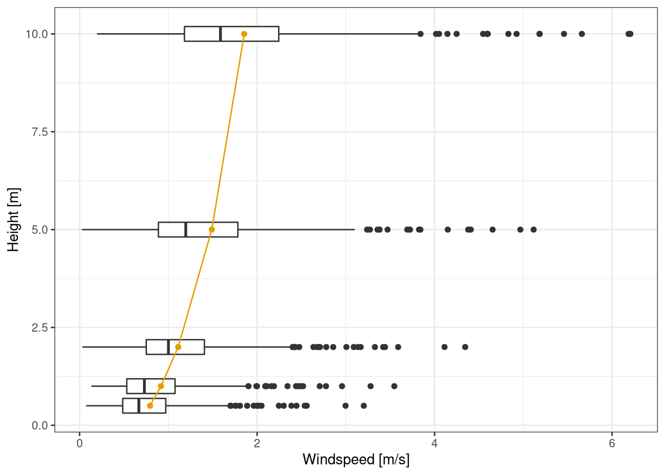

Figure 7.3: Distribution of daily means of wind speed at the different heights. The yellow line was obtaining by fitting a wind log profile to the mean of daily means. Data from botanical garden Jan 2020 - Feb 2021.

7.4.3 Windspeed over year

The wind rose for different quarters of the year are plotted (Figure 7.4) and then yearly pattern of wind speed and wind direction analyzed separately.

During the spring and winter the wind is stronger. In summer daily average oscillates around 1.5 m/s (Figure 7.5).

The graphs displays the variation of the wind speed along year. It is faster from end of December to beginning of April. During summer the mean wind speed is lower but some days it gets faster than others. This variability is originated depending on when the wind is coming from.

The wind direction is usually coming from overall the south (Figure 7.6) for the majority of th year, with the exception of the early summer where the north direction is also common. The reason why the prevalent winds are from the south is probably connected with the direction of the slope of the hill where the station is located, which is in the south direction.

wind_q <- wind %>% 
  mutate(quarter = quarter(Date),
         quarter = case_when(
           quarter == 1 ~ "Jan-Mar",
           quarter == 2 ~ "Apr-Jun",
           quarter == 3 ~ "Jul-Sep",
           quarter == 4 ~ "Oct-Dec",
         ))
windrose(wind_q$WS_10m, wind_q$wd, wind_q$quarter, n_col= 2, col_pal="YlGnBu",
         ggtheme = "bw")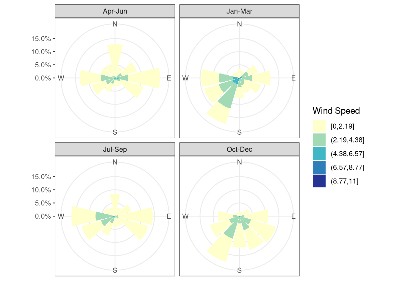

Figure 7.4: Wind rose for different quarters of the year. Data from botanical garden Jan 2020 - Feb 2021.

ggplot(wind_1d, aes(Date, WS_10m)) +
  geom_line() +
  labs(y="Wind speed (m/s)")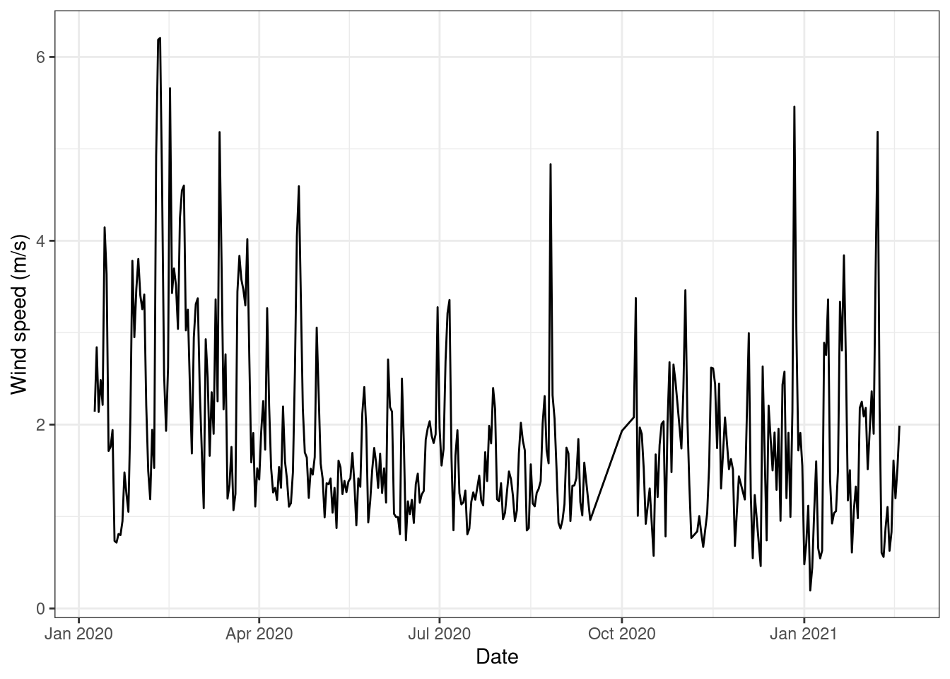

Figure 7.5: Daily averages of wind speed at 10 meters. Data from forest botanical garden January 2020 - February 2021.

# data frame with months start and end to draw background
months <- map_df(1:14, function(n_mon){
  start <- as_datetime("2020-01-01")
  # offset to the correct month start
  month(start) <- month(start) + n_mon - 1
  end <- start
  # adding one month to get to the end and removing one day
  month(end) <- month(end) + 1
  day(end) <- day(end) - 1
  tibble(start = start, end = end,
         month= month(start, label = T), quarter= quarter(start))
} )

wind %>%
  group_by(round_date(Date, unit = "1 weeks")) %>%
  summarise(across(c(matches("WS"), Date), mean), wd = wind_dir_average(wd)) %>% 
  ggplot() + 
  geom_rect( #add months in the background to be able to read the figure
    aes(xmin = start, xmax = end, fill = month), 
    ymin = -Inf, ymax = Inf, alpha = 0.6, 
    data = months
  ) +
  scale_fill_brewer(palette = "Set3") +
  geom_point(aes(Date, wd)) +
  coord_polar(theta="y") +
  labs(y="Wind direction", fill="Month") +
    scale_y_continuous(breaks = c(90, 180, 270, 360),
                     labels = c('E', 'S', 'W', 'N' ), limits=c(0, 360))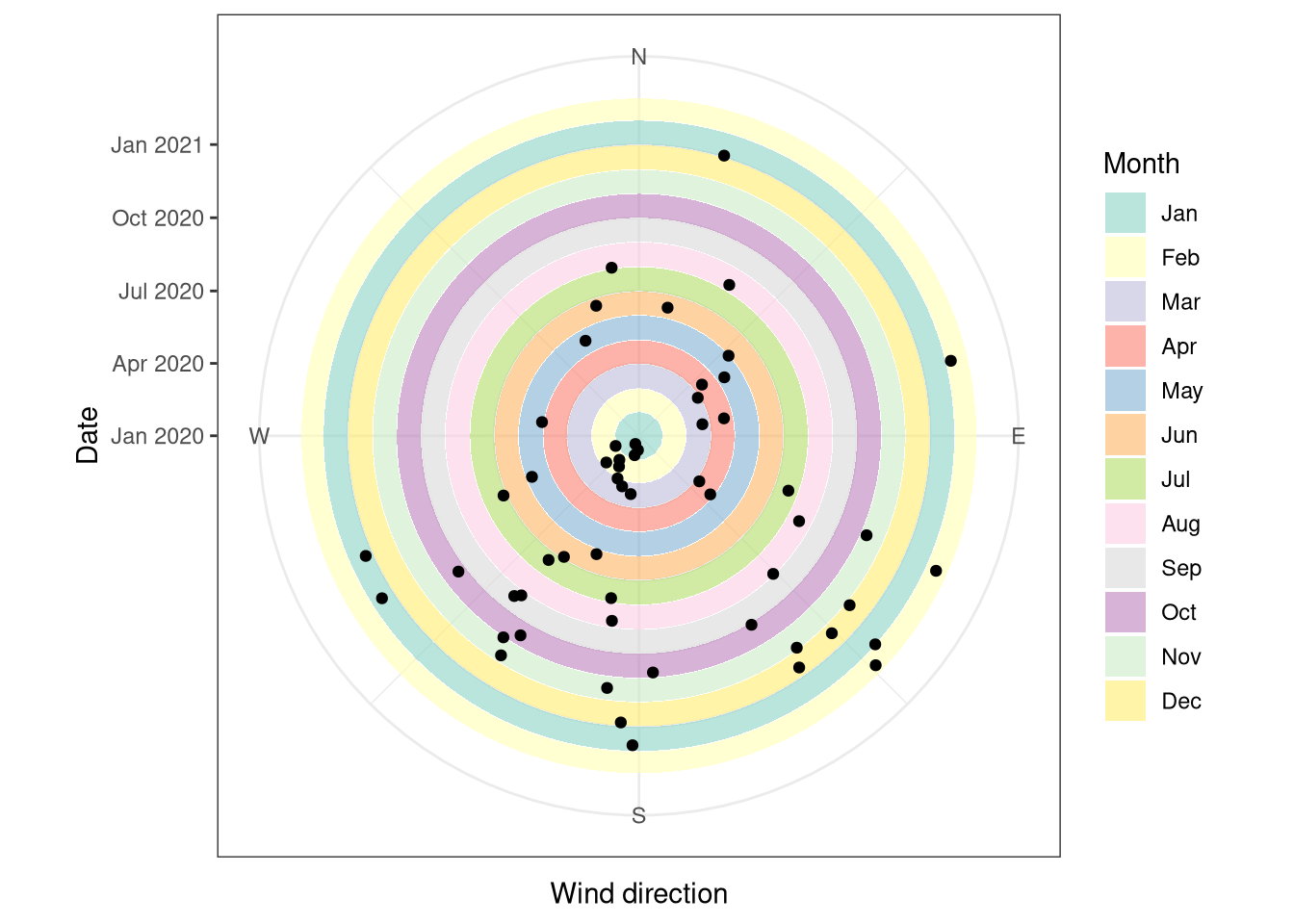

Figure 7.6: Weekly average of wind directions for the year (black dots). The distance from the center and the different background indicates the date, while the position in the circle the wind direction. Data from forest botanical garden January 2020 - February 2021.