10 Turbulent fluxes \(\pmb{CO_2}\)

10.1 Motivation

Part of the turbulent fluxes regulating the natural systems on earth is \(CO_2\) flux. In this chapter, we learned some ways to trace the flux of this important gas, also well known as green house gas. First, a small introduction about the carbon cycle in land ecosystems. Carbon approaches vegetation through the photosynthesis. Afterwards, carbon is allocated in different parts of plants; leafs, stem and root, while part of it is also lost by the leaching of soil and erosion. During the process of plant respiration, Carbon dioxide is also released in small amounts, together with the respiration of roots and other microorganisms present in soil. Although seems as a process easy to quantify, it also has its adversities, such as the turbulent movement of gas fluxes in forests.

10.2 Background

The measurement of the net \(CO_2\) exchange can be achieved by direct or continuous way, this way ecosystem is not disturbed. Also it can be measured by the integration over the entire ecosystem. Some researches have been going on measuring the carbon cycle at a global scale. This is known as the integrated carbon observation system (ICOS). The ICOS consists on the long term assessment of European carbon balance, with sample plots at different levels: atmosphere, terrestrial ecosystem and ocean. This programme is not the only one, also Fluxnet; measuring \(CO_2\), water vapor and energy flux all along the world. Thanks to these type of initiatives, other natural factors can be analyzed such as temperature, precipitation, temperature and soil moisture. As an example, the drought experienced in Europe in 2018, where a big decreasing in the \(CO_2\) uptake in central Europe was experienced, while and increase was observed in southern and northern countries of Europe. Besides the consequences of this drought period, the European average had a smaller effect than in 2003.

A simple definition of flux is the exchange of any quantity per area and time. The flux of \(CO_2\) and \(H_2O\) is measured with \(\mu mol\ m^{-2} s{-1}\) and \(mmol\ m^{-2} s{-1}\) respectively. Leaf evapotranspiration and Heat is measured by \(W m^{-2}\).

10.3 Sensors and measuring principle

The data measurement of gas fluxes can be done with the use of different ways, by data driven or with the use of instruments. Later, this data is required in ecosystem modelling. According to what flux is going to be measured, some instruments can be required as an additional equipment. The instruments can be: chambers, lysimeter and sap flow. The following formula describes the principle on which gas chambers are based on to measured \(CO_2\) flux in soil.

The \(CO_2\) flux assumption is based on its linear increase, using the following formula;

\[F_c = \frac{dc}{dt} \frac{MV}{A}\]

where:

\(dc\): change of \(CO_2\) concentration (\(\mu mol\ mol^{-1}\))
\(dt\): change in time (\(s\))
M = \(p / R\ T\) molar volume (\(mol\ m^{-3}\))
R = 8.314 \(J\ mol^{-1} K^{-1}\)
V: chamber volume (\(m^3\))
A: chamber surface area (\(m^2\))

10.4 Analysis

Calculate the half hourly latent heat flux, the net ecosystem exchange of \(CO_2\) and the sensible heat flux from the high frequency turbulence data.

library(tidyverse)
library(cowplot) #multiple plots
library(naniar) # to replace missing values 
library(ggthemes)
theme_set(theme_bw())

10.5 Respiration chambers

Field data were collected with respiration chambers. Four chambers were installed and for each of them the \(CO_2\) concentration measured roughly every 10 minutes.

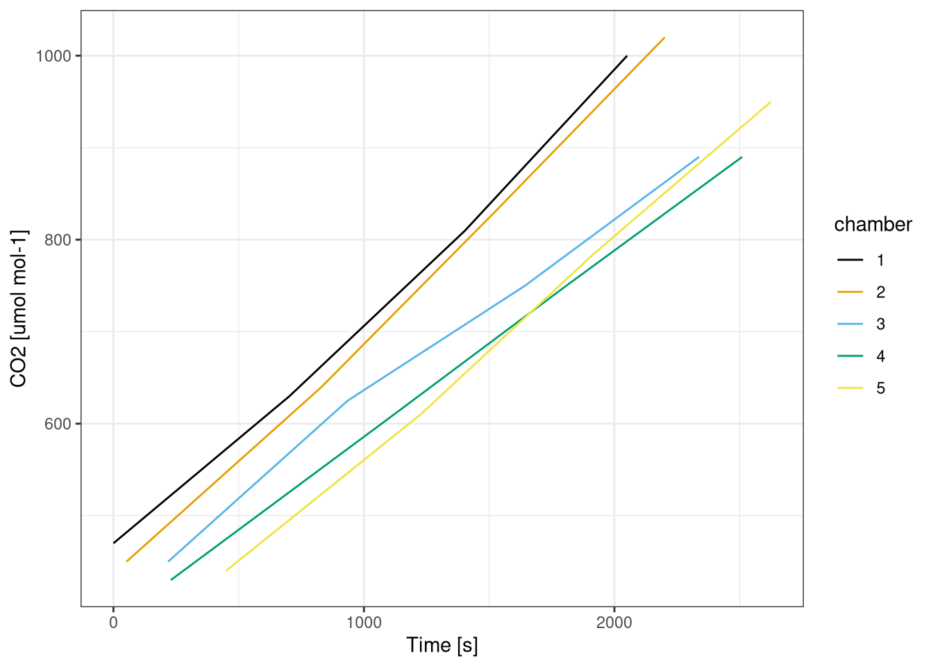
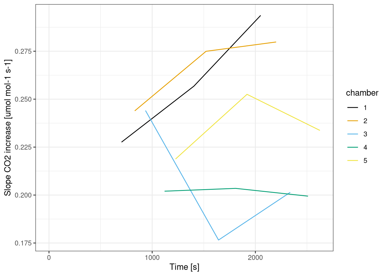
The \(CO_2\) concentration increase linearly over time (Figure 10.1) in all chamber, the slope of this increase is a bit different for each chamber and varies slightly with time, but is overall constant (Figure 10.2).

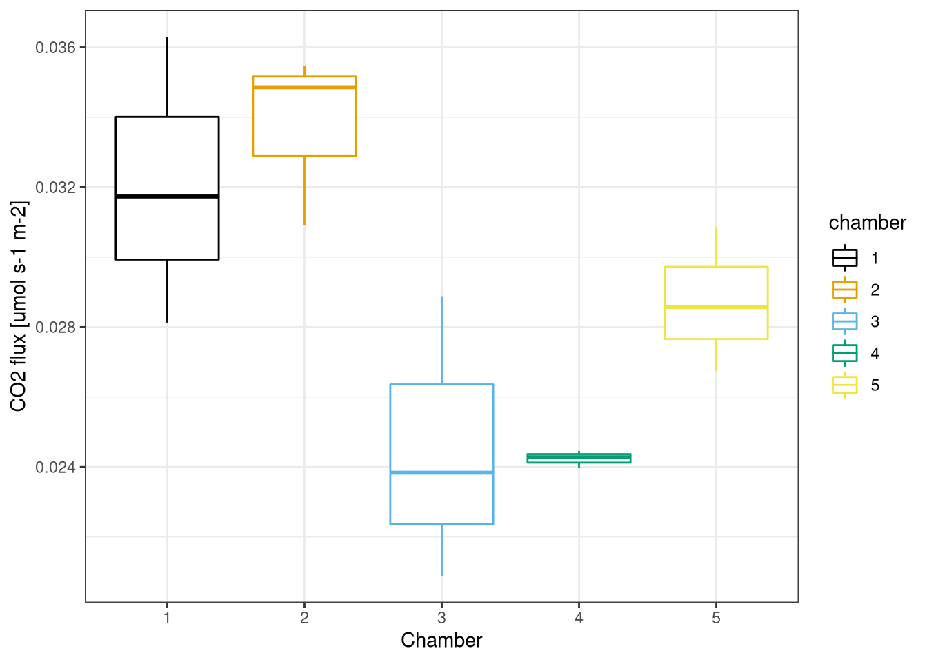
The \(Co_2\) flux is the computed (Figure 10.3). The Different chambers have different respiration rates, higher in 1 and 2, lower in 3 and 4 and intermediate in 5. The respiration between different chambers is overall comparable.

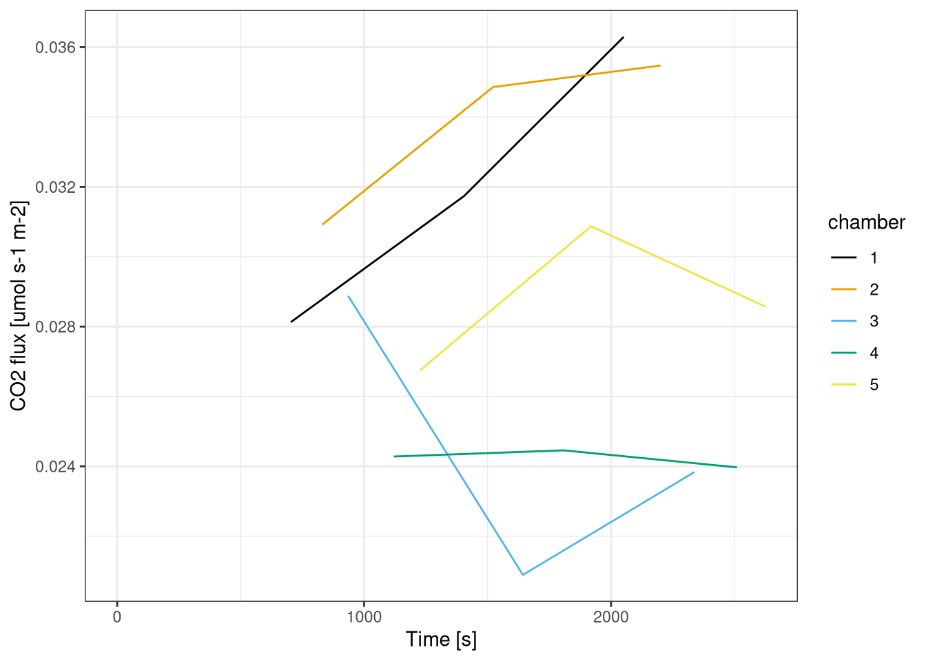
In Figure 10.4 the time flux over time is plotted. This is expected to be constant, but this is only the case for the chamber 4, that is very stable. For the other chambers there is a much higher variation and in particular in the first two chambers the flux increases over time. This is probably due to measurement errors as the field it was hard to estimate when the \(CO_2\) concentration in the chamber was stabilizing.

co2 <- read_csv2(here::here("Data_lectures/soilCO2flux.csv"),
                 col_names=c("time", "co2", "chamber"), skip=1)
# loading some data directly from in the R code for simplicity
p_a <- 989.5 #hPa - air pressure
T_a <- 16 + 273.15 # °C - air temperature
diam <- 0.152 # m - radius of chamber
top_height <- 0.138 # m - height of top part of the chamber (same for everything)

# area 
area <- pi / 4 *diam^2

# chamber specific data
chambers <- tribble(
  ~"Tsoil",~"chamber",~"height",
  17,     1, 0.16225,       
  17,     2, 0.17,
  16.8, 3, 0.1495,
  16.7, 4, 0.154,
  17.2, 5, 0.159
) %>% 
  mutate(
    Volume= pi / 4 * diam^ 2 * (height+top_height))
# Molar Gas Constant
R <- 8.314 # J/mol K

# Molar volume 
M <- p_a / (R*T_a)

co2flux <- co2 %>%
  # Adding chamber information
  left_join(chambers) %>% 
  group_by(chamber) %>% 
  mutate(
    dt = time - lag(time),
    dc = co2 - lag(co2),
    Fc = (dc/dt)*(M*Volume/area),
    # for plotting
    chamber = as.factor(chamber)
  )

ggplot(co2flux, aes(time, co2, col=chamber)) +
  geom_line() +
  scale_color_colorblind() +
  labs(x="Time [s]", y="CO2 [umol mol-1]")

Figure 10.1: Increase of \(CO_2\) concetration over time in each of the chamber. Data from field measurements.

ggplot(co2flux, aes(time, dc/dt, col=chamber)) +
  geom_line() +
  scale_color_colorblind() +
  labs(x="Time [s]", y="Slope CO2 increase [umol mol-1 s-1]")

Figure 10.2: Slope of the increase in \(CO_2\) concetration over time in each of the chamber. Data from field measurements.

ggplot(co2flux, aes(chamber, Fc, col=chamber)) +
  geom_boxplot() +
  scale_color_colorblind() +
  labs(x="Chamber", y="CO2 flux [umol s-1 m-2]")

Figure 10.3: \(CO_2\) flux measured in the different chambers. Data from field measurements.

ggplot(co2flux, aes(time, Fc, col=chamber)) +
  geom_line() +
  scale_color_colorblind() +
  labs(x="Time [s]", y="CO2 flux [umol s-1 m-2]")

Figure 10.4: \(CO_2\) flux measured in the different chambers over time. Data from field measurements.