3 Air temperature

3.1 Motivation

Temperature is arguably the environmental variable with the biggest impact of ecosystems. The speed of all chemical reactions is strongly influenced by temperature in a non-linear way, therefore processes like photosynthesis and respiration shows an strong response to temperature changes. Moreover, thermal energy is the main way ecosystem can store energy, hence the temperature constantly change to maintain energy balance. Finally the temperature often influences water availability.

3.2 Background

Temperature is defines as a state variable, which describes the mean kinetic energy of molecules. The SI unit to measure temperature is the Kelvin degree K, that use a reference point the absolute zero, the temperature when there is no motion of molecules.

Often other measurement units are used mainly degrees Celsius (°C) and Fahrenheit (°F).

In a gas the temperature is related to the pressure by the ideal gas law:

\[pV = nRT\] Therefore in the troposphere there is a drop in temperature with height, as the pressured is reduced with height.

3.3 Sensors and measuring principle

Temperature is measured using different principles, for analog sensors the the measures are connected to thermal expansion of materials. The increase in temperature results in an increase of volume or length and its magnitude on the materials properties. In particular the most common sensors are:

• Mercury Thermometer. The sensor has a bulb filled with mercury (or other liquid) that expands or contracts with the change in temperature, that is then connect to a graded pipe where is possible to make the reading.

• Bimetal Thermometer. The sensor is based on the different expansion coefficient of metals, hence by putting two different metals (eg. iron and copper) next to each other the temperature can be measured by the amount of the bent.

• Thermocouple. Thermocouples measure the voltage at the junction of two metals, which in turn depends on temperature.

• Resistance. They measure the change in resistance due to the change of temperature. There are two types of sensors with diffenrt type of responses,

  • Positive temperature coefficient (PTC). Increase Usually made of platin.
  • Negative temperature coefficient (NTC). Decrease the resistance with an increase in temperature, they are usually made of semi conductors

3.4 Analysis

3.4.1 Hainich time series

temp <- read_csv(here("Data_lectures/3_Air_temperature/Hainich_T_air_soil_degC.csv")) %>% 
  mutate(diff_canopy = TA_44m - TA_2m) %>% 
  drop_na()

The temperature changes at different height of the canopy, due to the different incoming solar radiation and emitted longwave radiation. Similarly the top soil temperature can be significantly different from the air temperature just above the soil, this is due to the higher heat capacity and lower conductivity of the soil compared to the air. In this analysis the air temperature at 2 meters is compared with the temperature 2 cm below the soil.

The soil temperature daily variation is limited compared to the air one (Figure 3.1 and 3.2). In one day the air temperature can change up to 10 °C, while the soil temperature only a few degrees. However, over the year the total variation of air and soil temperature are similar (Figure 3.1). Moreover also the yearly mean are similar (Table 1).

In general the air and the soil temperature follow a similar pattern, but the daily oscillation in the air temperature are bigger (Figure 3.3).

temp %>% 
  group_by(Date = round_date(Date, "1d")) %>% 
  summarize_all(mean) %>% 
  ggplot(aes( x = Date)) +
  geom_line(aes(y=Tsoil_002m_degC, col="Soil 2 cm")) +
  geom_line(aes(y=TA_2m, col="Air 2 meters")) +
  scale_color_colorblind() +
  labs(y = "Temperature [°C]", col="Heigth")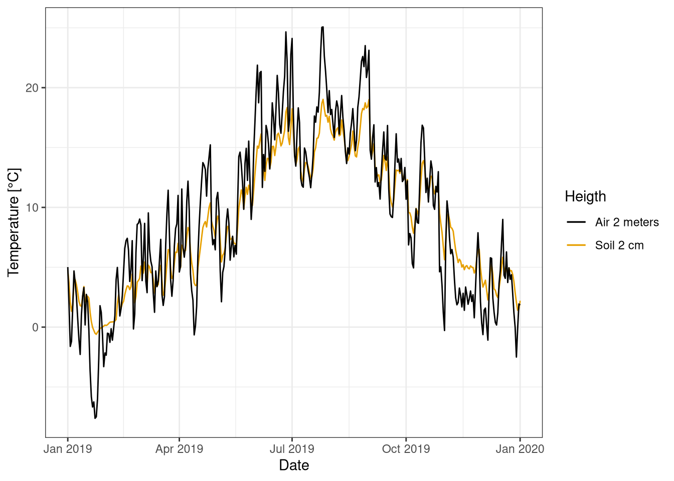

Figure 3.1: Comparison time series temperature at 2 m and 2 cm in the soil for 2019. Measurement averaged over 1 day. Data from Hainich national park

temp %>% 
  filter(between_dates(Date, "1 May 2019", "30 May 2019")) %>% 
  ggplot(aes(Date)) +
  geom_line(aes(y=Tsoil_002m_degC, col="Soil 2 cm")) +
  geom_line(aes(y=TA_2m, col="Air 2 meters")) +
  scale_color_colorblind() +
  labs(y = "Temperature (°C)", col="Heigth")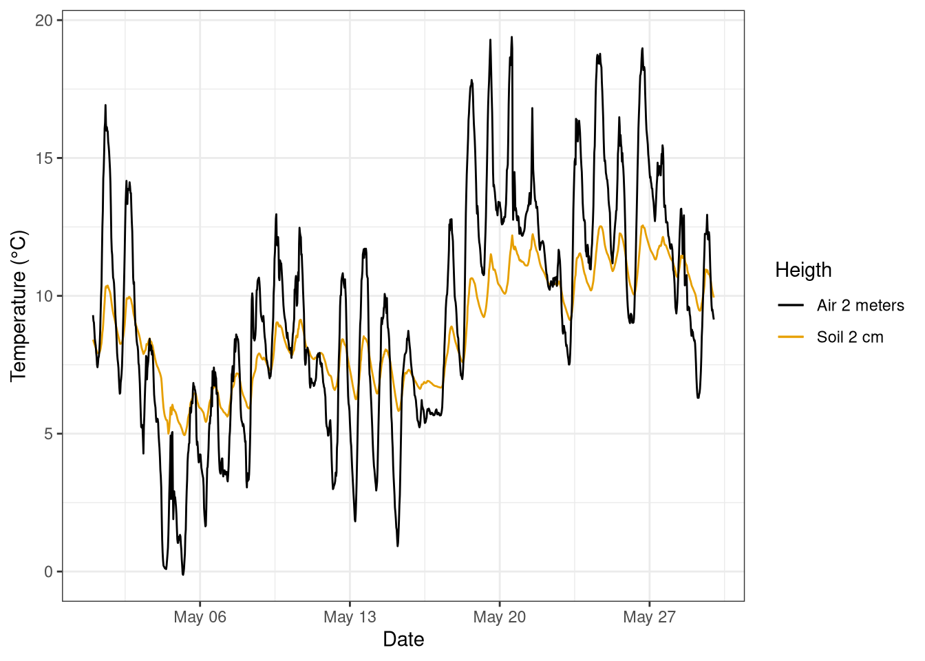

Figure 3.2: Comparison time series temperature at 2 m and 2 cm in the soil for the month of May 2019. measurement frequency 30 min. Data from Hainich national park

temp %>% 
  group_by(Date = round_date(Date, "1d")) %>% 
  summarize_all(mean) %>% 
  ggplot(aes(TA_2m, Tsoil_002m_degC)) +
  geom_point() +
  scale_color_colorblind() +
  geom_smooth(method = "lm", se=F, colour = colorblind_pal()(2)[2]) +
  labs(x="Temperature air 2m [°C]", y = "Temperature soil 2cm [°C]")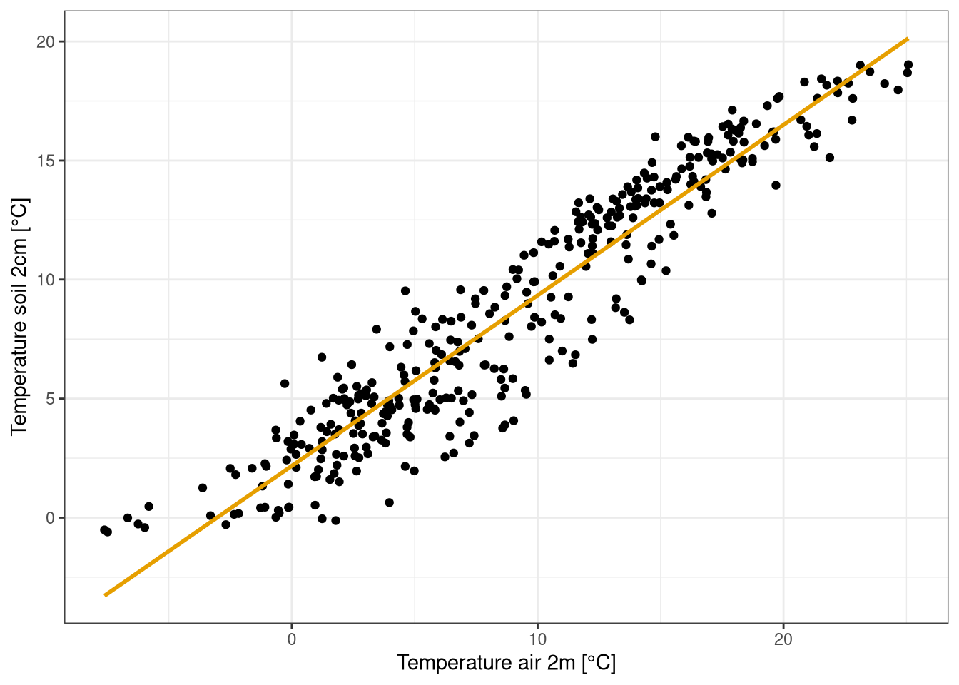

Figure 3.3: Scatter plot with regression line between temperature at 2 m and 2 cm in the soil for 2019. measurement averaged over 1 day. Data from Hainich national park.

tribble( ~"Variable", ~"Value",
  "Correlation air and soil temperature", cor(temp$TA_2m, temp$Tsoil_002m_degC),
  "Mean temperature air", mean(temp$TA_2m),
  "Mean temperature soil",  mean(temp$Tsoil_002m_degC)) %>% 
  kable(booktabs=T, caption="Summary soil and air temperature") %>% 
  kable_styling(latex_options = "hold_position")

Table 3.1: Summary soil and air temperature

Variable	Value
Correlation air and soil temperature	0.9287618
Mean temperature air	9.1323011
Mean temperature soil	8.7184121

3.4.2 Temperature sensors response time

The goal of the field experiment is to estimate the response time of a resistance thermometer and a mercury one.

To estimate the response time we can start from the following equation that describes the temperature decrease over time. Then this can be inverted and used to estimated by \(\tau\) fitting a linear model.

\[T_t = T_a + (T_0 - T_a) e^{\frac{T} {-\tau}}\]

In the field the sensors where heated up and then the temperature measured every 10 seconds while they cooled down. The air temperature was also recorded for reference.

res_wire <- 3.7 # Omega. This has been measured in the field
r_0 <- 100 # Omega at 100 degrees
a <- 4e-3

#' converts resistance to temperature
get_temp <- function(resistance) {
  (((resistance - res_wire) / 100) - 1) / 4e-3 
}

temp_res <- read.csv(here("3_air_temperature/resistance_sensor_cooling response.csv"),
                     header = T)

# add the time (in seconds) and the temperature after conversion from resistance
temp_res <- temp_res %>%
  mutate(time = 0:(nrow(temp_res)-1) * 10,
         temp = get_temp(resistance) )

T_a <- 13.0 # calculations done in the field
T_0 <- temp_res$temp[1] # first measure 

temp_res <- temp_res %>% 
  mutate(log_t = log((T_0 - T_a) / (temp - T_a)) )

model_res <- lm(time ~ log_t, data=temp_res)

ggplot(temp_res, aes(time, temp)) +
  geom_line() +
  labs(y = "Temperature [°C]", x = "Time [s]")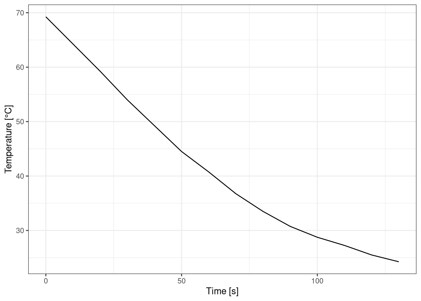

Figure 3.4: Temperature decrease over time for resistance thermometer.

temp_merc <- read.csv(here("3_air_temperature/mercury_termometer_cooling_response.csv"),
                      header = T)

T_a <- 7.0 # ambient temperature
T_0 <- temp_merc$temp[1] # first measure 

temp_merc <- mutate(temp_merc, log_t = log((T_0 - T_a) / (temp - T_a)) )

model_merc <- lm(time ~ log_t, data=temp_merc)

ggplot(temp_merc, aes(time, temp)) +
  geom_line() +
  labs(y = "Temperature [°C]", x = "Time [s]")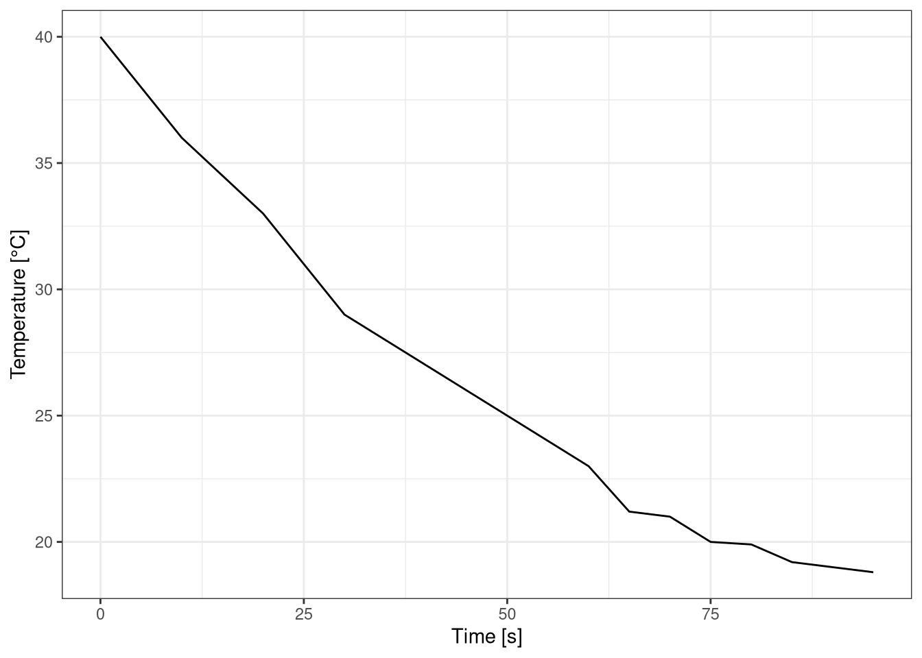

Figure 3.5: Temperature decrease over time for mercury thermometer.

The time response rate for the resistance sensor is 77 seconds.

The time response rate for the mercury sensor is 88 seconds.

The mercury thermometer has an higher response time than the resistance one.

This is against the expectations as the mass, and therefore the thermal inertia, of the mercury sensor is smaller than the resistance one.