11 Turbulent Fluxes Eddy Covariance

11.1 Motivation

The atmosphere and the ecosystem exchange energy and gases through turbulent flows. The main gas transported are $CO_2$ and water vapour, while energy is transferred as sensible heat fluxes and momentum fluxes.

Eddy Covariance (EC) is a technique that measures the entity of the turbulent fluxes. It can measure a wide range of variables, automatically, continuously, with high accuracy and with minimal impact on the ecosystems. It is primary method used to monitor the carbon balance of ecosystems.

11.2 Background

The air flow next to the surface becomes turbulent, with eddies that transport mass and energy between the atmosphere and the ecosystems. It is possible to measure the properties of the eddies and use them to estimate the different fluxes. Therefore in an Eddy Covariance setup the first instrument needed is an anemometer that measures the 3 components of the wind, this can then be paired with a gas analyzer to measure the change of concentration. The fluxes can then be calculated as the covariance between the vertical wind and the property of interest.

In particular those are the most common fluxes that are measured:

$\pmb{CO_2}$. Carbon dioxide is one of the main variable measured in EC setups, as it is the main outcome of photosynthesis and respiration. The flux can be calculated as:

\[F_{co2} = \rho_m\overline{w`c_{co2}`}\] where $\rho_m$ is the air molar density and $\overline{w`c`}$ the covariance between the vertical wind speed (w) and the $CO_2$ concentration. The measurement unit is $\mu mol / m^2s$.

$\pmb{H_2O}$. The amount of water vapour exchanged can be The flux can be calculated as:

\[E_{h2o} = \rho_m\overline{w`c_{h2o}`}\] where $\rho_m$ is the air molar density and $\overline{w`c`}$ the covariance between the vertical wind speed (w) and the H2O concentration. The measurement unit is $\mu mol / m^2s$.

Latent heat. Latent heat flux is the amount of energy that is transferred due the evaporation of water vapour. In fact it is directly connected to the $H_2O$ flux and can be calculated as:

\[LE = \lambda E\] where $\lambda$ is the latent heat of vaporization of water and $E$ is the $H_2O$ flux.

The unit of measurement is $W/m^2$

Sensible heat. The sensible heat flux is the amount of energy exchanged as heat. The heat energy can be transferred through the movement of air masses. The flux can be calculated as:

\[H = \rho_a c_p \overline{w`T`}\] where $\rho_a$ is the air density, $c_p$ is the air heat capacity and $\overline{w`T`}$ the covariance between the vertical wind speed (w) and T the air temperature. The measurement unit is $W / m^2$.

Momentum. Momentum is the amount of mechanical energy that is transferred from the wind to the ecosystem. It is by definition negative, as the the ecosystem cannot transfer mechanical energy to the wind.

The flux can be calculated using only measures from a 3D anemometer as:

\[\tau = \rho_a \sqrt{(\overline{w`u`})^2 + (\overline{w`v`})^2}\] where $\rho_a$ is the air density and $u$ and $v$ the two horizontal wind components. The measurement unit is $Kg / ms^2$.

The Eddy Covariance technique is very powerful, however, flux calculation are based on several assumptions and require complex post processing to reduce the errors.

First of all Eddy covariance can be applied only when there is a well developed turbulent layer, which is often not the case at night. Then measurements in heterogenous enviroments or on slopes can affect the turbulence and hence the flxes measurers.

The EC data needs to be preprocessed to remove instruments errors (despiking and calibration) and compensate for non ideal instrument setup (time lag correction, coordinate rotations). Flux can then be calculated for a time period and then additional correction applied due to the loss of high frequency information (spectral corrections) and change in gas density (Webb-Pearmen-Leuning correction).

Each instrument and variable need to have each of the steps mentioned above tailored for its specific characteristics.

11.3 Sensors and Measuring principles

Eddies have different sizes and speed but many of them are small and very fast (fraction of seconds), therefore instruments with high response rate are needed.

A basic EC setup consist of two instruments, an anemometer and a gas analyzer. The anemometer is a 3D sonic anemometer, that can therefore also measure the vertical component of the wind and have high frequency reading. The gas analyzer measure the concentrations using the absorption of specific infrared wavelenghts. The most commonly measured gas are $CO_2$, $H_2O$ and methane. Gas analyzer can be open path, where the measurement chamber is directly exposed to the air or closed path where the measure take place in a separate chamber and the air is pumped through a pipe.

The EC instruments are mounted on a tower as they need to be above the ecosystem where the turbulence layer is well developed.

11.4 Analisys

ec_col_names <-  c("TIMESTAMP","TIMESTAMPS","u","v","w","T_sonic",
                   "SA_DIAG_VALUE","CO2_ABS","H2O_ABS","CO2_CONC",
                   "H2O_CONC","CO2_POW_SAM","H2O_POW_SAM","CO2_POW_REF",
                   "H2O_POW_REF","co2","h2o","T_CELL","PRESS_CELL",
                   "GA_DIAG_CODE","T_DEW","CO2_STR")

ec_test_path <- 
  "Data_lectures/10_Turbulent_fluxes_II/10_Turb_fluxes_CO2/Reinshof_flux_HF_202105300001.dat" %>% 
  here::here()
ec <-read_csv(ec_test_path, skip=4, col_names = ec_col_names, na=c("", "NaN"))

files <- dir_ls(here::here("Data_lectures/10_Turbulent_fluxes_II/10_Turb_fluxes_CO2/"))

# taking 4 sample data for plots at 4 different moment of the day
# need to convert integer and remove the last element
idx <- seq(1, 48, length.out=10) %>% as.integer() %>% head(-1)
ec_samples_paths <- files[idx]
ec_samples <- map(ec_samples_paths,
                  ~read_csv(.x, skip=4, col_names = ec_col_names, na=c("", "NaN")))

11.4.1 Raw flux calculation

The fluxes are first calculated without applying any correction.

# the emp
process_ec_file <- function(file, p=function(){}) {
  ec <-read_csv(file, skip=4, col_names = ec_col_names, col_types = cols(), na=c("", "NaN"))
  time <- str_extract(file, "\\d+.dat$") %>% 
    parse_date_time("YmdHM")
  flux <- calc_fluxes(ec) %>% 
    mutate(time = time)
  p() # step progress bar
  return(flux)
}

# Molar Gas Constant
R <- 8.314 # J/mol K

#' Calcuates all fluxes
calc_fluxes <- function(ec){
  # celsius to kelvin
  T_a <- ec$T_CELL + 273.15
  # need to convert pressure to Pa from kPa
  p_a <- ec$PRESS_CELL * 1e3
  
  # how to calc this?
  rho_a <- 1
  # How to calc lambda 
  # how to calc Cp

  tibble(
    rho_m = calc_rho_m(p_a, T_a),
    co2 = calc_co2_flux(ec$w, ec$co2, rho_m),
    h2o = calc_h2o_flux(ec$w, ec$h2o, rho_m),
    sens_heat = calc_sens_heat_flux(ec$w, ec$T_sonic, rho_a),
    lat_heat = calc_lat_heat_flux(h2o),
    mom = calc_mom_flux(ec$u, ec$v, ec$w, rho_a)
  )
}

calc_co2_flux <- function(w, co2, rho_m){
  cov(w, co2, use="complete.obs") * rho_m
}

calc_h2o_flux <- function(w, h2o, rho_m){
  cov(w, h2o, use="complete.obs") * rho_m
}

calc_mom_flux <-  function(u, v, w, rho_a){
  sqrt(
    cov(w, u, use="complete.obs")^2 * cov(w, v, use="complete.obs")^2
  ) * rho_a
}

calc_sens_heat_flux <- function(w, T_sonic, rho_a, Cp= 1000){
  cov(w, T_sonic, use="complete.obs") * rho_a * Cp
}

calc_lat_heat_flux <- function(h2o_flux, lambda = 2.256 ) {
  h2o_flux * lambda
}

# air molar density
calc_rho_m <- function(p, T_a){
  mean( p / (R * T_a), na.rm=T)
}

files <- dir_ls(here::here("Data_lectures/10_Turbulent_fluxes_II/10_Turb_fluxes_CO2/"))
with_progress({
  # this is to have a progress bar
  p <- progressor(along=files)
  ec_flux <- cache_rds(map_dfr(files, process_ec_file, p))
})

11.4.2 Flux corrections

In order to properly measure the fluxes several corrections are necessary. In the subsequent section the main correction are analyzed individually and tested then the fluxes with the corrections are calculated.

11.4.2.1 Remove implausible values

The first step is not a proper correction, but a plausibility check. All the readings outside sensible ranges are discarded. To test this function some artificial data has been generated and as seen in Table 11.1 the out of range values were correctly removed.

remove_implausible <- function(ec){
  ec %>% 
    replace_with_na_at(c("u", "v", "w"), ~abs(.x) > 10) %>% 
    replace_with_na_at("co2", ~!between(.x, 350, 700)) %>% 
    replace_with_na_at("T_sonic", ~!between(.x, -15, 50)) %>% 
    replace_with_na_at("h2o", ~!between(.x, 2, 30))
}

# manually checking with some fake data that the function is working as intended
tibble(
  u = seq (-15, 15, length.out=20),
  v = u,
  w = u,
  co2 = seq (30, 800, length.out=20),
  T_sonic = seq (-20, 80, length.out=20),
  h2o = seq (0, 40, length.out=20),
) %>% 
  remove_implausible() %>% 
  kbl(booktabs=T, caption="Example dataset after removal of implausible values") %>% 
  kable_styling(latex_options = "hold_position")

Table 11.1: Example dataset after removal of implausible values
u	v	w	co2	T_sonic	h2o
NA	NA	NA	NA	NA	NA
NA	NA	NA	NA	-14.736842	2.105263
NA	NA	NA	NA	-9.473684	4.210526
NA	NA	NA	NA	-4.210526	6.315790
-8.6842105	-8.6842105	-8.6842105	NA	1.052632	8.421053
-7.1052632	-7.1052632	-7.1052632	NA	6.315790	10.526316
-5.5263158	-5.5263158	-5.5263158	NA	11.578947	12.631579
-3.9473684	-3.9473684	-3.9473684	NA	16.842105	14.736842
-2.3684211	-2.3684211	-2.3684211	354.2105	22.105263	16.842105
-0.7894737	-0.7894737	-0.7894737	394.7368	27.368421	18.947368
0.7894737	0.7894737	0.7894737	435.2632	32.631579	21.052632
2.3684211	2.3684211	2.3684211	475.7895	37.894737	23.157895
3.9473684	3.9473684	3.9473684	516.3158	43.157895	25.263158
5.5263158	5.5263158	5.5263158	556.8421	48.421053	27.368421
7.1052632	7.1052632	7.1052632	597.3684	NA	29.473684
8.6842105	8.6842105	8.6842105	637.8947	NA	NA
NA	NA	NA	678.4211	NA	NA
NA	NA	NA	NA	NA	NA
NA	NA	NA	NA	NA	NA
NA	NA	NA	NA	NA	NA

11.4.2.2 Despike

Despiking consists in removing spikes in the data, which are moment where suddenly very different. Here the spikes are considered as the values where the different from the mean is bigger than a certain number of times (default 5) the standard deviation. This is a simple despiking method and the number should be properly tuned for each measured variable according to their characteristics and sensor behavior.

Figure 11.1 shows how this despiking filter works. The limit of 1.8 standard deviations is artificially low and used in the plot only as an example of the deskipe. All the values that are outside the range mean +/- 1.8 standard deviation are removed and replaced with NAs.

despike <- function(data, times_sd = 5) {
  mean_data <- mean(data, na.rm=T)
  sd_data <- sd(data, na.rm=T)
  spikes <- abs(data - mean_data) > (times_sd*sd_data)
  # spikes will be NAs
  data[spikes] <- NA
  return(data)
}

plots_despike <- map(ec_samples, function(ec){
  co2_mean <- mean(ec$co2, na.rm=T)
  co2_sd <- sd(ec$co2, na.rm=T) * 1.8
  ggplot(ec, aes(TIMESTAMP, despike(co2, times_sd = 1.8))) +
    geom_hline(yintercept = co2_mean) +
    geom_hline(yintercept = c(co2_mean + co2_sd, co2_mean - co2_sd), linetype=2) +
    geom_line(aes(y = co2), color="grey60") +
    geom_line(colour = colorblind_pal()(2)[2]) +
    labs(x="Time", y="CO2 [umol mol-1]")
})

do.call(plot_grid, c(plots_despike[c(1, 3, 6, 9)], nrow=2))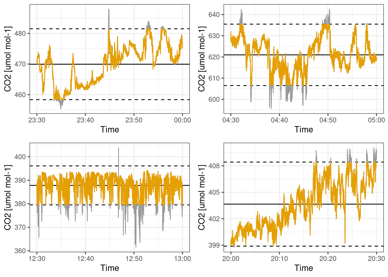

Example of how despiking work with articially low factor of +/- 1.8 standard deviations. Grey sections is the data that was removed. Dashed lines are the mean +/- 1.8 standard deviation. Each subplot is a different time of the day. Data from Hainich national park 31st May 2021.

Figure 11.1: Example of how despiking work with articially low factor of +/- 1.8 standard deviations. Grey sections is the data that was removed. Dashed lines are the mean +/- 1.8 standard deviation. Each subplot is a different time of the day. Data from Hainich national park 31st May 2021.

11.4.2.3 Rotations

The reference system of the wind is rotated in order to have a zero mean in the vertical wind component and a zero mean wind direction.

Table 11.2, shows the values of the wind means before and after the double rotation, which works correctly.

# wind should have 3 columns u, v, and w
double_rotation <- function(wind){
  
  wind %>% 
    # 1st rotation around z into the mean wind direction
    mutate(
      # need to use atan2 otherwise the angle may have the wrong sign
      theta = atan2(mean(v,na.rm = T), mean(u,na.rm = T)),
      u_1 = u*cos(theta) + v*sin(theta),
      v_1 = -u*sin(theta) + v*cos(theta),
      w_1 = w
    ) %>%
    # 2nd rotation around new y-axis to nullify the vertical wind speed
    # to be used for further analysis
    mutate(
      phi = atan2(mean(w_1,na.rm = T), mean(u_1,na.rm = T)),
      u_2 = u_1*cos(phi) + w_1*sin(phi),
      v_2 = v_1,
      w_2 = -u_1*sin(phi) + w_1*cos(phi)
    ) %>% 
    # rename variables
    mutate(
      u = u_2,
      v = v_2,
      w = w_2) %>% 
    # remove temp variables
    select(
      -u_1, -v_1, -w_1, -theta, -phi, 
    )
}

rot_wind <- double_rotation(ec)

tribble(~"Variable", ~"Before correction", ~"After correction",
  "Mean vertical wind", mean(ec$w), mean(rot_wind$w),
  "Mean wind direction", mean(atan2(ec$v, ec$u)), mean(atan2(rot_wind$v, rot_wind$u))) %>% 
  kbl(booktabs = T, caption="Mean wind speed and direction before and after double rotation") %>% 
  kable_styling(latex_options = "hold_position")

Table 11.2: Mean wind speed and direction before and after double rotation
Variable	Before correction	After correction
Mean vertical wind	-0.0136382	0.0000000
Mean wind direction	1.9793592	0.0005655

11.4.3 Time lag correction

Due to spatial separation between the gas analyzer and the anemometer each Eddy is measured at slightly different moments in time, this difference even if it often very small can lead to serious underestimation of fluxes. Therefore a time lag correction has been developed to compensate this. For each variable and half an hour a time lag is calculated in order to maximize the correlation between the vertical wind speed and the gas concentration. This is done by trying different time lags and then finding the one where the absolute correlation is maximized.

# maybe find a better name, lag that supports negative values
lag2 <- function(x, n){
  if (n >= 0){
    lag(x, n)
  }
  else{
    lead(x, -n)
  }
}

#lags the second argument
lagged_cor <-  function(x, y, n){
  cor(x, lag2(y, n), use="complete.obs")
}

max_n_cor <- function(w, gas){
  # maximise the absolute value of the covariance
  opt <- optimize(function(n){
    # the optimize function use doubles, leg uses ints
    abs(lagged_cor(w, gas, as.integer(n)))
  }, interval = c(-700, 700), maximum = T, tol=1)
  return(opt$maximum)
}

time_lag_correction <- function(w, gas){
  lag2(gas, max_n_cor(w, gas) %>% as.integer )
}

Figure 11.2 show the time log correction for the $CO_2$ sensor. As it can been seen during the day (7h - 17h) there is a clear peak in the correlation plot and the time lag found by the optimization algorithm is in a sensible range. However during night the is no peak and the found time lag is outside a sensible range. This is probably due to the fact that at night the turbulent fluxes are not well developed and therefore it is difficult to correctly apply EC. In order to better test this hypothesis in figure 11.3 the time lag correction has been applied to the the sonic temperature, where it should be 0 as it is measured together with the wind speed. The time lag correction is correctly found to be 0 during the day, but not for the night. This confirms that the time lag correction is working properly and the problem is related to the fluxes themselves.

In real life conditions more complex algorithm and quality assurance system are used to avoid this kind of errors.

plots_lag <- map(ec_samples, function(ec){
  co2_lagged_cor <- tibble( n = seq(-700, 700, 5), 
                         lagged_cor = map_dbl(n,~ lagged_cor(ec$w, ec$co2, .x)))
  max_cor <- max_n_cor(ec$w, ec$co2) %>% round(0)
  ggplot(co2_lagged_cor, aes( x= n , y = lagged_cor)) +
    geom_line() +
    geom_vline(xintercept = max_cor, col=colorblind_pal()(2)[2]) +
    labs(title=ec$TIMESTAMP[1] %>% 
           format("%Hh%M") %>% 
           paste(" lag:", max_cor), y="correl", x="time lag")
})

do.call(plot_grid, c(plots_lag))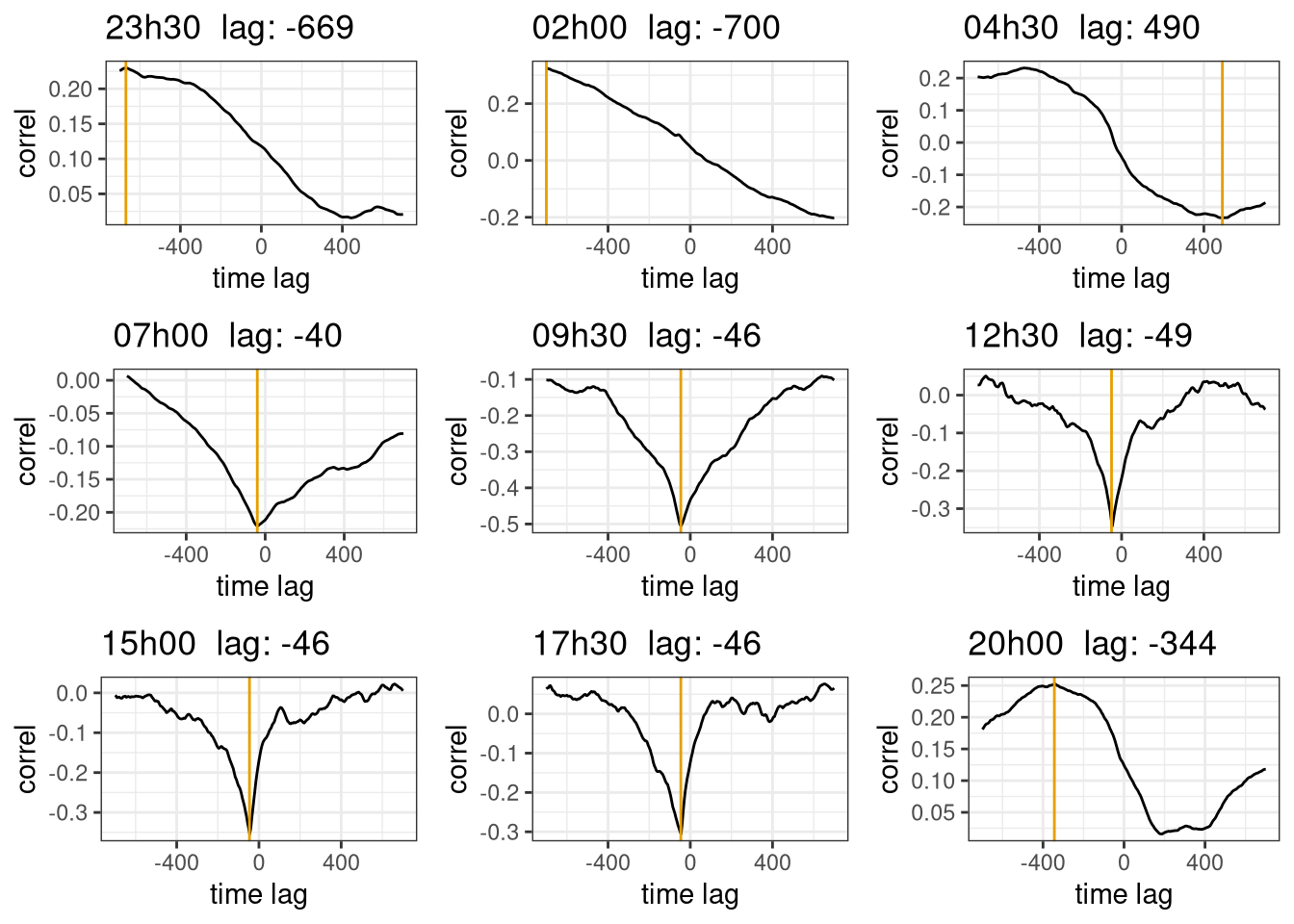

Time lag correction for $CO_2$. The plots are the correlation coefficient with different time lags, the yellow line is at the max value found by the optimization algorithm. The subplot are for different time of the day. Data from Hainich national park first week June 2021.

Figure 11.2: Time lag correction for $CO_2$. The plots are the correlation coefficient with different time lags, the yellow line is at the max value found by the optimization algorithm. The subplot are for different time of the day. Data from Hainich national park first week June 2021.

plots_lag <- map(ec_samples, function(ec){
  co2_lagged_cor <- tibble( n = seq(-700, 700, 5), 
                         lagged_cor = map_dbl(n,~ lagged_cor(ec$w, ec$T_sonic, .x)))
  max_cor <- max_n_cor(ec$w, ec$T_sonic) %>% round(0)
  ggplot(co2_lagged_cor, aes( x= n , y = lagged_cor)) +
    geom_line() +
    geom_vline(xintercept = max_cor, col=colorblind_pal()(2)[2]) +
    labs(title=ec$TIMESTAMP[1] %>% 
           format("%Hh%M") %>% 
           paste(" lag:", max_cor), y="correl", x="time lag")
})

do.call(plot_grid, c(plots_lag))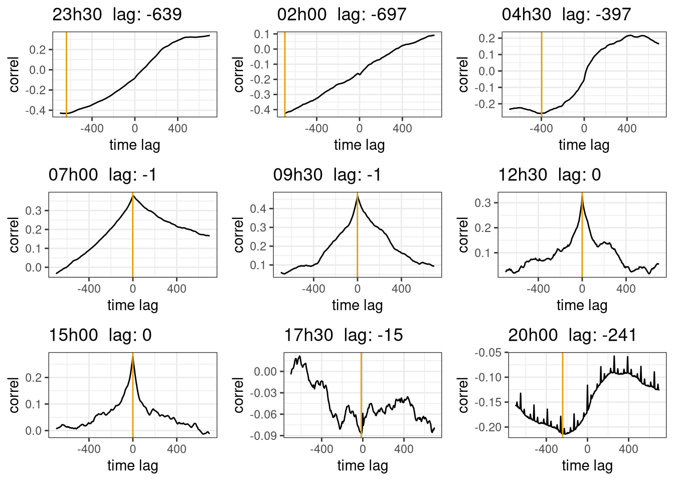

Time lag optimization for sonic temperature. The expected time lag optimization is 0 as the sonic temperature is measured by the anemometer itself. The plots are the correlation coefficient with different time lags, the yellow line is at the max value found by the optimization algorithm. The subplot are for different time of the day. Data from Hainich national park first week June 2021.

Figure 11.3: Time lag optimization for sonic temperature. The expected time lag optimization is 0 as the sonic temperature is measured by the anemometer itself. The plots are the correlation coefficient with different time lags, the yellow line is at the max value found by the optimization algorithm. The subplot are for different time of the day. Data from Hainich national park first week June 2021.

11.4.4 Corrected fluxes

All the correction are applied to the fluxes calculations and each variable is analyzed.

apply_corr <- function(ec){
  ec %>% 
    #remove_implausible() %>% # this step is very slow and not really needed.
    mutate(across(c(u, v, w, co2, h2o, T_sonic), despike)) %>% 
    double_rotation %>%
    mutate(across(c(co2, h2o), ~time_lag_correction(w, .x)))
}

process_ec_file_corr <- function(file, p=function(){}) {
  ec <-read_csv(file, skip=4, col_names = ec_col_names, col_types = cols(), na=c("", "NaN"))
  time <- str_extract(file, "\\d+.dat$") %>% 
    parse_date_time("YmdHM")
  flux <- ec %>% 
    apply_corr %>% 
    calc_fluxes %>% 
    mutate(time = time)
  p() # step progress bar
  return(flux)
}

files <- dir_ls(here::here("Data_lectures/10_Turbulent_fluxes_II/10_Turb_fluxes_CO2/"))

with_progress({
  # this is to have a progress bar
  p <- progressor(along=files)
  ec_flux_corr <- cache_rds(map_dfr(files, process_ec_file_corr, p))
})

11.4.4.1 $\pmb{CO_2}$ fluxes

The $CO_2$ flux (Figure 11.4) has a clear daily pattern, negative during the day and positive during the night. This is expected as during the day there is photosynthesis and $CO_2$ is absorbed by plants resulting in an overall negative flux, while during the night there is only respiration that produces positive $CO_2$ fluxes.

The importance of correction can also be seen with the raw fluxes underestimating the $CO_2$ flux. This is striking on the 30 of May and is mainly due to the missing time lag correction.

ggplot() +
  geom_hline(yintercept = 0, linetype=2) +
  geom_line(aes(time, co2, col="raw"), data = ec_flux) +
  geom_line(aes(time, co2, col="corrected"), data= ec_flux_corr) +
  scale_color_colorblind() +
  labs(x="Time", y="CO2 flux [umol m-2 s-1]", col="Flux")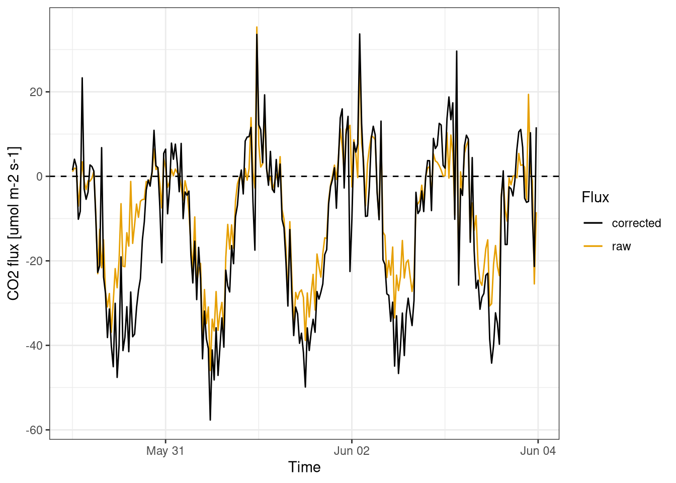

$CO_2$ fluxes. Comparison between corrected and raw fluxes calculations. Fluxes calculated for every half an hour. Data from Hainich national park first week June 2021.

Figure 11.4: $CO_2$ fluxes. Comparison between corrected and raw fluxes calculations. Fluxes calculated for every half an hour. Data from Hainich national park first week June 2021.

11.4.4.2 $\pmb{H_2O}$ fluxes

The water fluxes have also a a daily pattern (Figure 11.5), with the majority of the water exchanged during the day from the ecosystem to the atmosphere. The evapotraspiration of water during the day is the process that drives the fluxes.

In this figure 11.5 the importance of water flux correction is evident.

ggplot() +
  geom_hline(yintercept = 0, linetype=2) +
  geom_line(aes(time, h2o, col="raw"), data = ec_flux) +
  geom_line(aes(time, h2o, col="corrected"), data= ec_flux_corr) +
  scale_color_colorblind() +
  labs(x="Time", y="H2O flux [mmol m-2 s-1]", col="Flux")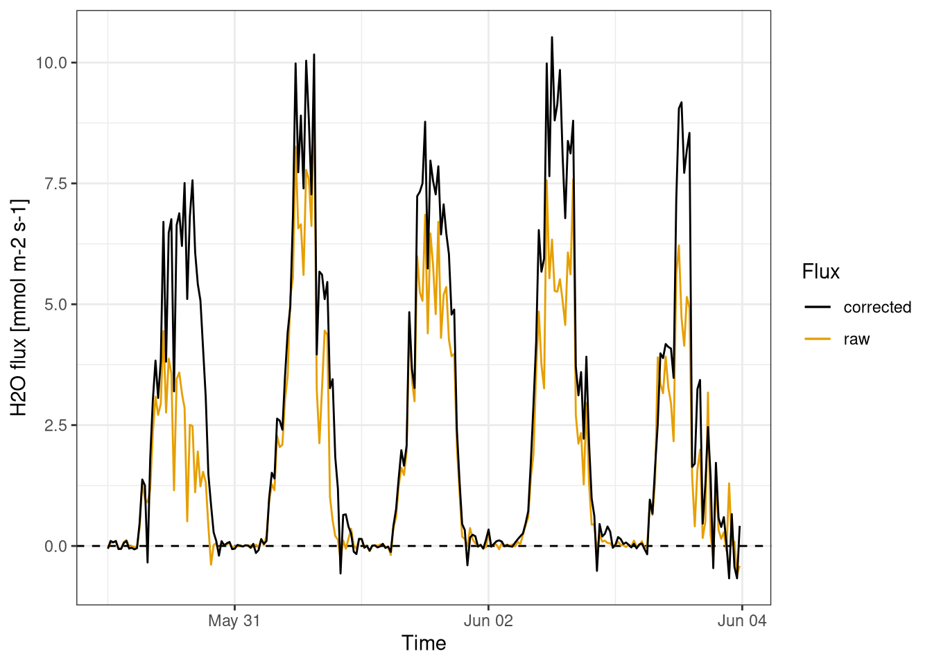

$H_2O$ fluxes. Comparison between corrected and raw fluxes calculations. Fluxes calculated for every half an hour. Data from Hainich national park first week June 2021.

Figure 11.5: $H_2O$ fluxes. Comparison between corrected and raw fluxes calculations. Fluxes calculated for every half an hour. Data from Hainich national park first week June 2021.

11.4.4.3 Latent heat fluxes

The latent heat flux (Figure 11.6) is by definition has the same pattern of water vapour fluxes.

ggplot() +
  geom_hline(yintercept = 0, linetype=2) +
  geom_line(aes(time, lat_heat, col="raw"), data = ec_flux) +
  geom_line(aes(time, lat_heat, col="corrected"), data= ec_flux_corr) +
  scale_color_colorblind() +
  labs(x="Time", y="Latent heat flux [W m-2]", col="Flux")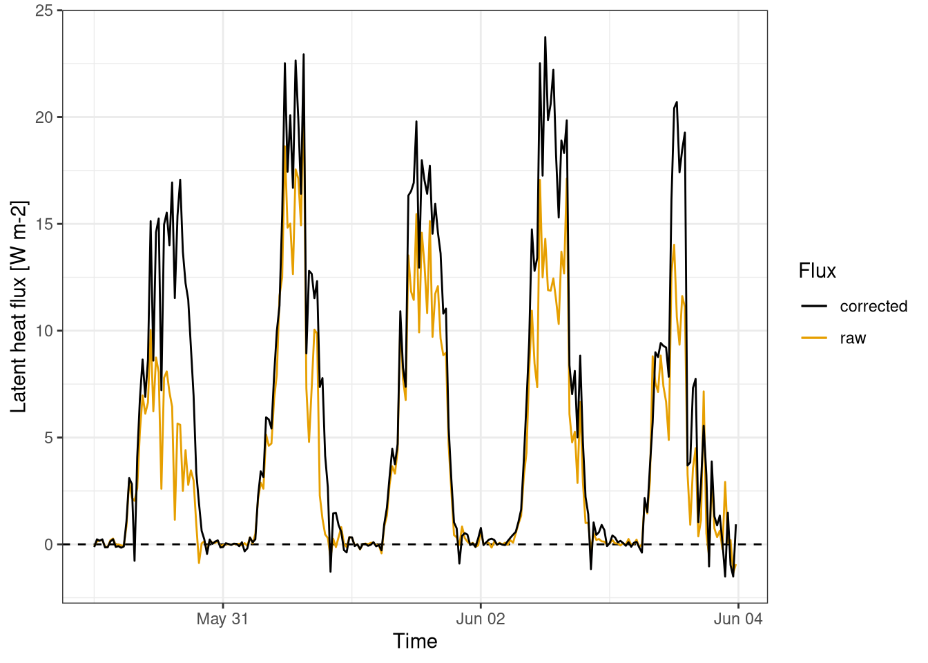

Latent heat fluxes. Comparison between corrected and raw fluxes calculations. Fluxes calculated for every half an hour. Data from Hainich national park first week June 2021.

Figure 11.6: Latent heat fluxes. Comparison between corrected and raw fluxes calculations. Fluxes calculated for every half an hour. Data from Hainich national park first week June 2021.

11.4.4.4 Sensible heat fluxes

The sensible heat flux (Figure 11.7) is driven the the different temperature between the surface and the atmosphere. During the day the surface heats up due to the incoming solar radiation and transfers the energy to the atmosphere. During the night the situation is often the inverse, but the amount of the flux is dependend on the weather conditions of each day.

The calculation of the sensible heat flux doesn’t require a gas a analyzer as the air temperature is measured by the sonic anemometer, hence there is no time lag and the entity of the flux correction is limited.

ggplot() +
  geom_hline(yintercept = 0, linetype=2) +
  geom_line(aes(time, sens_heat, col="raw"), data = ec_flux) +
  geom_line(aes(time, sens_heat, col="corrected"), data= ec_flux_corr) +
  scale_color_colorblind() +
  labs(x="Time", y="Sensible heat flux [W m-2]", col="Flux")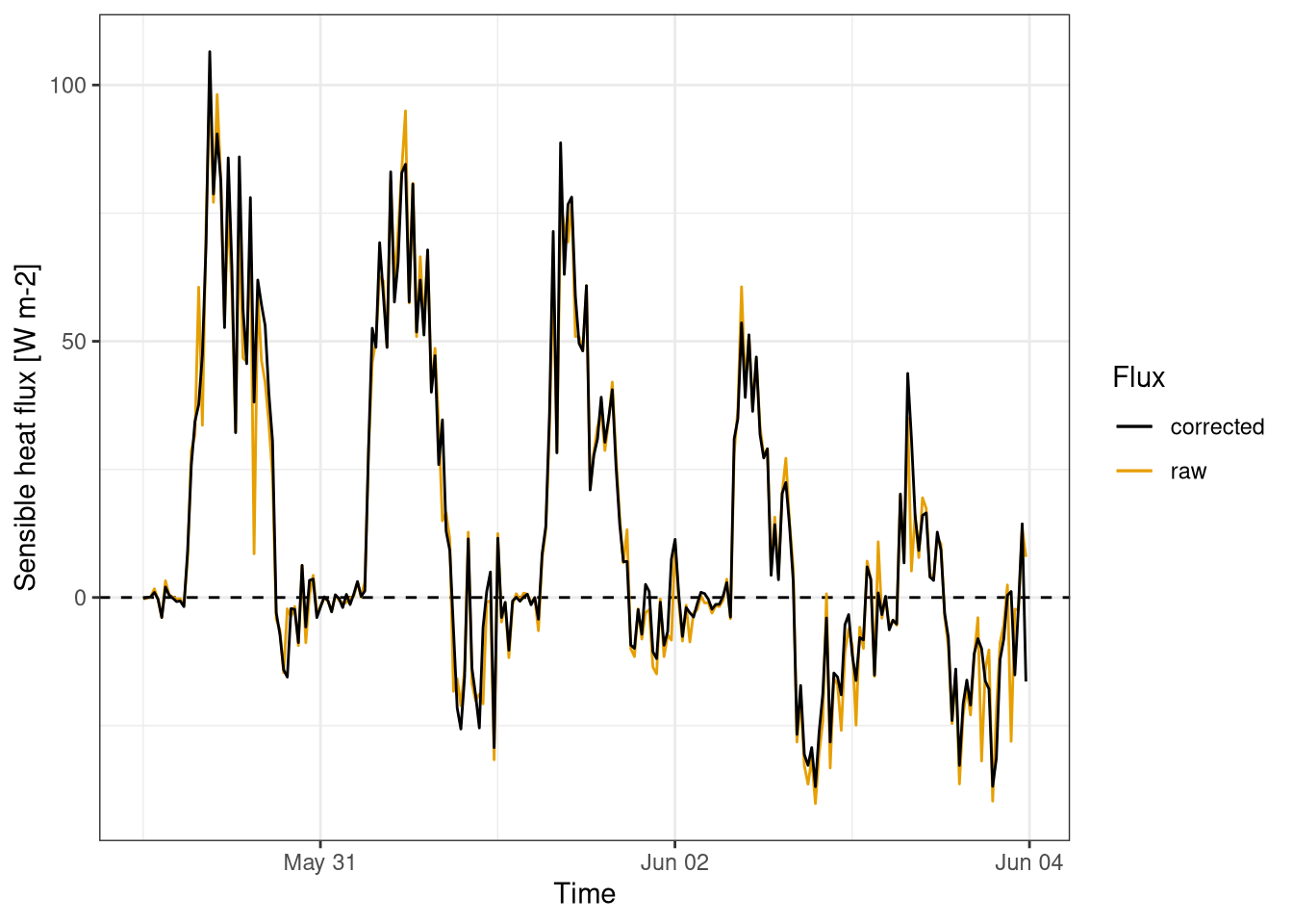

Sensible heat fluxes. Comparison between corrected and raw fluxes calculations. Fluxes calculated for every half an hour. Data from Hainich national park first week June 2021.

Figure 11.7: Sensible heat fluxes. Comparison between corrected and raw fluxes calculations. Fluxes calculated for every half an hour. Data from Hainich national park first week June 2021.

11.4.4.5 Momentum fluxes

The momentum flux (Figure 11.8) is dependent on the wind speed, that is often higher during the afternoons and very low during the night. Moreover the flux is always positive, as expected.

The main flux correction relevant to the momentum is the coordinate rotation, as there is not time lag. The raw fluxes are often significantly different from the corrected ones.

ggplot() +
  geom_line(aes(time, mom, col="raw"), data = ec_flux) +
  geom_line(aes(time, mom, col="corrected"), data= ec_flux_corr) +
  scale_color_colorblind() +
  labs(x="Time", y="Momentum flux [kg m-1 s-2]", col="Flux")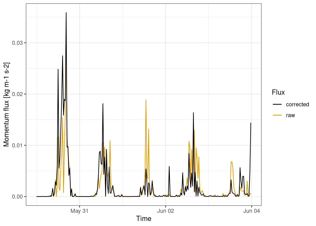

Momentum fluxes. Comparison between corrected and raw fluxes calculations. Fluxes calculated for every half an hour. Data from Hainich national park first week June 2021.

Figure 11.8: Momentum fluxes. Comparison between corrected and raw fluxes calculations. Fluxes calculated for every half an hour. Data from Hainich national park first week June 2021.

Experimental bioclimatology Term Paper