1 Shortwave radiation
1.1 Motivation
The sun is the source of all energy reaching the Earth. It arrives under the form of electromagnetic radiation, in particular of light in the shortwave range.
The incoming shortwave radiation heats up the surface and the atmosphere with different intensity. This is the core reason behind numerous phenomena on the earth, from seasons to winds. Moreover a small fraction of shortwave radiation is captured by the plants through photosynthesis, its converted to chemical energy and it is the basis for the whole biosphere.
1.2 Background
Electromagnetic radiation are oscillations of a magnetic and electric field. Electromagnetic radiation is formed by waves, that have a characteristics wavelength and frequency.
Electromagnetic radiation is a form of energy, hence it is measured in Joule (\(J\)) and its intensity Watts (\(J/s = W\)).
Every body emits electromagnetic radiation, the intensity and the wavelength of the emitted radiation depends on its temperature and is described by Planck’s law.
Due to its temperature the sun emits short-wave radiation, that have a wavelength in the range \((0.2 - 4) \mu m\).
Solar radiation is composed by ultraviolet radiation with a wavelenght lower than \(0.4 \mu m\), visible radiation \((0.4-0.7) \mu m\) and near-infrared \(>0.5 \mu m\).
In contrast with sun radiation, the radiation emitted by objects in earth will not surpass the range of \(3-100 \mu m\), and this ratio is known as long wave radiation or infrared.
Stefan-Boltzmann law describes the total amount of radiation emitted from bodies at a specific temperature. This law consists on the calculation of emittance (L) in (\(W / m^2\)) produced equal the product of the Stefan-Boltzmann constant (\(\sigma= 5.67 10 ^{-8} \frac{W}{m^2} K^{-4}\)) and the emissivity (\(\varepsilon\));
\[L= \varepsilon \sigma T^4\]
The emissivity as \(\varepsilon\) “the ratio of the actual emittance to the blackbody emittance”. A blackbody is described as the body that absorbs and emits all the radiation (Bonan 2019)
The solar radiation reaches the ecosystems and it is divided in 3 components: reflected, absorbed and transmitted. The amount of radiation in each of this component depends on the properties of the canopy and on the wavelength (\(\lambda\)). The following equation is true:
\[1= \sigma(\lambda)+r(\lambda)+t(\lambda)\] where:
Adsorption \(\sigma(\lambda)\) is the fraction of light that it blocked and absorbed by the medium.
Reflectivity \(r(\lambda)\) is the fraction of electromagnetic wave that is reflected backward. The reflectivity of a surface is also called albedo (Perkins 2019).
Transmissivity \(t(\lambda)\) is the fraction of energy going through a medium without experimenting any change.
Incoming shortwave radiation is formed by two different components:
Direct solar radiation (\(S\)): is the incident radiant flux density falling into a horizontal surface which will differ with the position of the sun.
Diffuse solar radiation (\(D\)): the incident radiant flux density arriving to the surface of earth after scattered and reflected during its way by other molecules as well present in air.
Global radiation (\(G\)): is the sum of diffuse and direct solar radiation.
\[ G = S + D \]
1.3 Sensors and measuring principle
Shortwave solar radiation can be measured with the use of different instruments that use different priciples. The main ones are:
Pyrheliometer: allows the direct measurement of shortwave radiation coming directly from the sun. It is disposed by a sensor that reacts at wavelengths around 0.2-4 micrometers. It needs to be set close to a sun tracker, this way it is possible to follow the movement of sun along day.
Pyranometer: this instrument measured the global shortwave radiation including the reflected shortwave radiation. It is based on the use of a sensor sensible at same wavelengths as the pyrheliometer, although in this case it must be parallel to the soil surface (horizontal). If the shortwave reflected needs to be measure, the sensor would need to be turn downwards facing the surface. In the case of Pyranometer, it is also used to measure diffused shortwave radiation. For this function, a shadow ring is set, normally shifting towards the suns azimuth angle during time. The main principle is the calculation of voltage differences with wires made of different methals. Normally these voltages are small, this is why the application of a thermopile. In order to decrease the error that winds and air temperature may induce, a glass is situated around the detector.
PAR Quantum sensor: this sensor is used for the measurement of Photosynthetically Active Radiation, it is more sensitive than the other with a range between 400-700 nm. It is formed by a filter on top of the sensor and a photodiode semiconductor made out of silicon. This way, incident light makes react the semiconductor, current measured in voltages with the used of resistance.
Campbell-Stokes sunshine autograph: this instrument is used to measure the sunshine duration of days. A circumference made of glass burns a paper where the sunshine time period is register.
1.4 Analysis
library(tidyverse)
library(ggplot2)
library(lubridate)
library(here)


shortwavedata <- read.csv(
  here("1_shortwave/Exercise_1st_lect/Shortwave_incoming_diffuse_W_m-2_Hainich_2020.csv"),
  header = TRUE, sep = ",")
shortwavedata$Date<- as.POSIXct(shortwavedata$Date, format= "%Y-%m-%d %H:%M")

calib_factorsdata <- read.csv(
  here("1_shortwave/Exercise_1st_lect/Shortwave_incoming_outgoing_belowcanopy_mV_Hainich_2020.csv"))
calib_factorsdata$Date<- as.POSIXct(calib_factorsdata$Date
                                    , format= "%Y-%m-%d %H:%M")

sw_b <- data.frame(
  Date = calib_factorsdata$Date,
  incoming = calib_factorsdata$Shortwave_incoming_mV * 86.5801,
  #mV *( W m-2 )/mV  = W m-2
  outgoing =  calib_factorsdata$Shortwave_outgoing_mV * 86.5801,
  #mV *( W m-2 )/mV  = W m-2
  belowcanopy = calib_factorsdata$Shortwave_incoming_bewlow_canopy_mV*194.9318
  #mV *( W m-2 )/mV = W m-2
)

# This is a quick hack to remove incorrect data when the radiation is low
sw_b[sw_b$incoming<=10 | sw_b$outgoing <=10 | sw_b$belowcanopy <= 10,] <- NA
sw_b <- drop_na(sw_b)
1.4.1 Albedo
The albedo is the fraction of incoming solar radiation that is reflected upwards by the earth surface (Figure 1.1). During the winter there are some peaks in the albedo and can be explained by measurement errors due to the low amount of radiation. The albedo is relatively constant across the year, in the range 10-17%. During the summer the albedo is higher, due to the higher reflectance of the green canopy compared to the dark ground.
sw_b <- mutate(sw_b,
               albedo = outgoing/incoming,
               transmitted = belowcanopy/incoming,
               absorbed = 1 - albedo)

sw_b_d <- sw_b %>%
  group_by(yday(Date)) %>%
summarise_all(mean)ggplot(sw_b_d, aes(x=Date))+
geom_line(aes(y=albedo)) +
labs(y = "Albedo", x = "Time")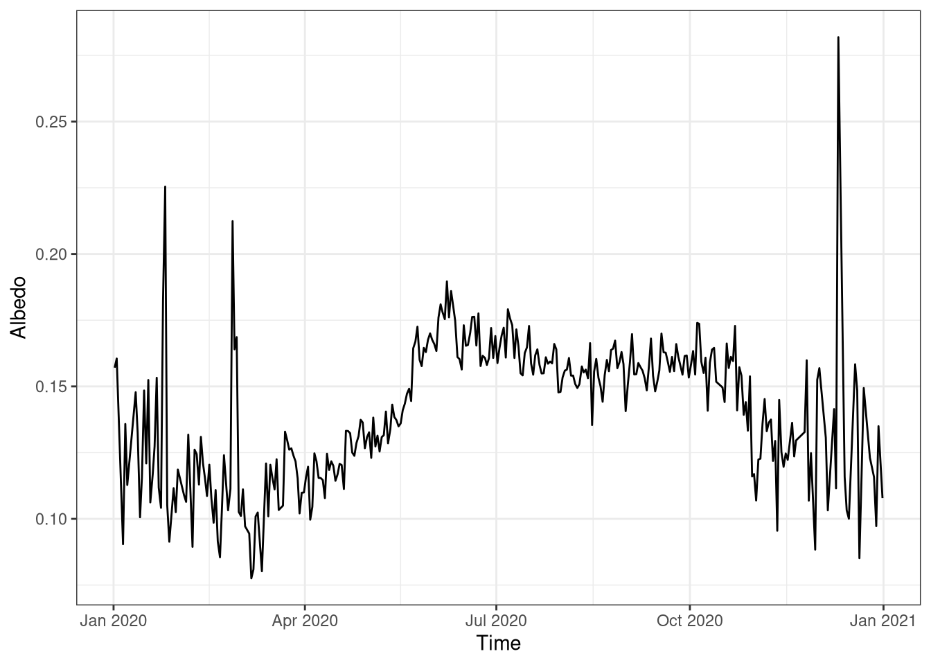
Figure 1.1: Surface albedo over the year. Data is averaged daily. Data from Hainich national park 2020.
1.4.2 Absorption coefficient
The Absorption coefficient is the fraction of incoming radiation that is absorbed by the ecosystems (Figure 1.2).
The absorption is quite constant, but during winter is higher (up to 90%) to then decrease in summer when there are leaves (83%). The peaks during the winter can be connected to measurement errors due to the low amount of radiation.
ggplot(sw_b_d, aes(x=Date))+
  geom_line(aes(y=absorbed))+
  labs(y = "Absorption coefficient", x = "Time") +
  ylim(0,1)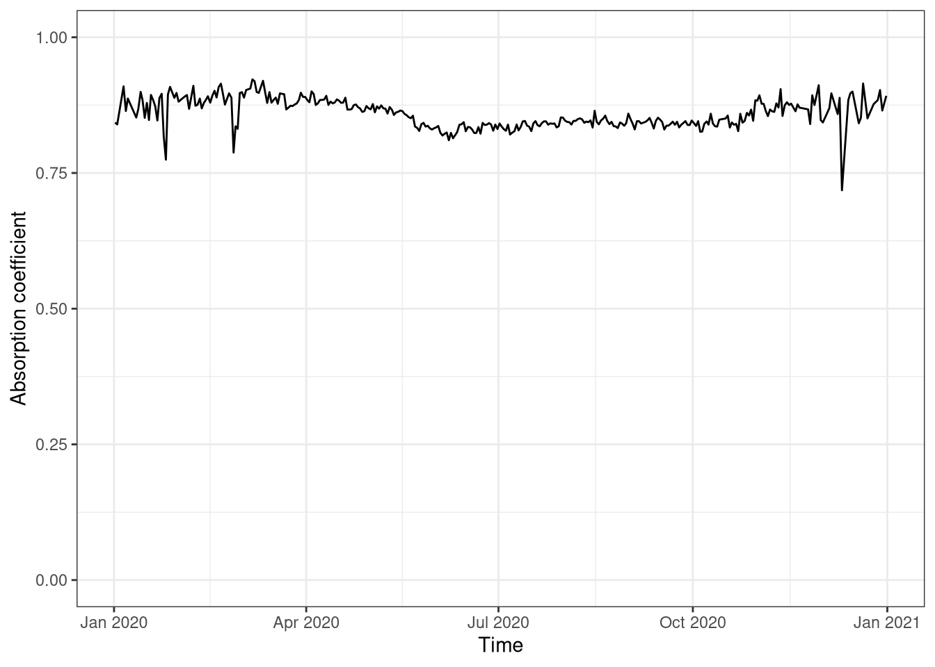
Figure 1.2: Absorption coefficient over the year, daily average. Data from Hainich national park 2020.
1.4.3 Transmission coefficient
The Transmission coefficient is the fraction of light that is transmitted through the canopy and reach the ground below (Figure 1.3).
During the year there is a clear difference between summer and winter. During winter the transmission is around 30% while during summer it is around 5%. This shows how effective are the trees in capturing available light.
ggplot(sw_b_d, aes(x=Date))+
  geom_line(aes(y=transmitted))+
  labs(y = "Trasmission coefficient", x = "Time") +
  ylim(0,.5)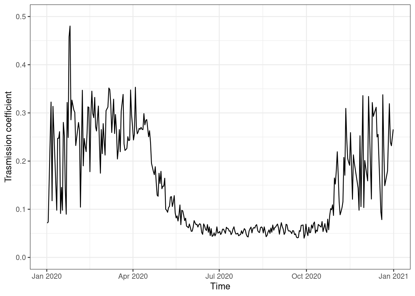
Figure 1.3: Absorption coefficient over the year, daily average. Data from Hainich national park 2020.
During summer days there is a daily cycle of the transmission coefficient (Figure 1.4). It is lower during the morning and evening and higher in the middle of the day. This can be explained because when the sun is low on the horizon there is more reflection and the light penetrates less in the canopy, thus resulting in a reduced transmission coefficient.
sw_b %>%
  filter(between(Date, as_datetime("2020-07-1"), as_datetime("2020-07-2"))) %>%
ggplot(aes(x=Date))+
  geom_line(aes(y=transmitted))+
  labs(y = "Trasmission coeficient", x = "Time")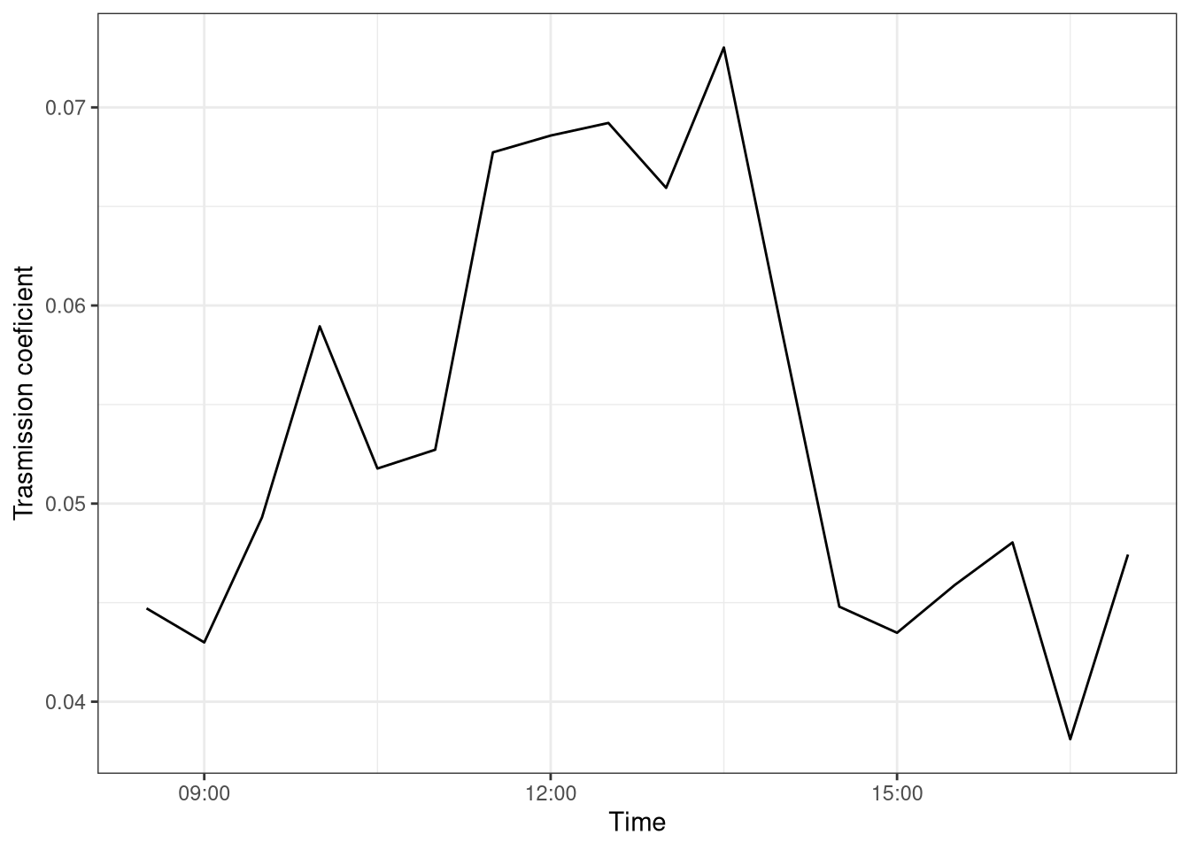
Figure 1.4: Daily cycle trasmittion coefficient. Data every 30 mins. Data from Hainich national park 1st July 2020.
1.4.4 Radiation below canopy
The absolute value of the radiation below the canopy (Figure 1.5) is relatively constant between summer and winter with the notable exception of spring. There are no leaves in the canopy yet, but the solar radiation is getting stronger. This can explain the why in beech forest there is a some undergrowth only during spring.
ggplot(sw_b_d, aes(x=Date))+
  geom_line(aes(y=belowcanopy))+
  labs(y = "Transmitted radiation [W m-2]", x = "Time")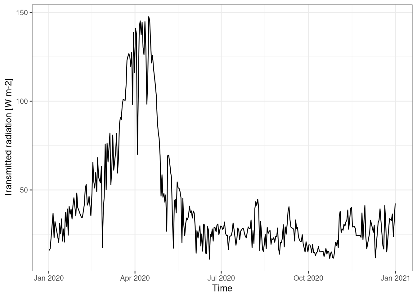
Figure 1.5: Radiation trasmitted below the canopy over the year. Data is averaged daily. Data from Hainich national park 2020.
1.4.5 Diffuse and direct radiation
The total radiation is sum of the diffuse and direct (Figure 1.6). The amount of direct radiation changes a lot during the year. You can see that April and September were relatively sunny months (direct and total radiation are similar), while July and August were cloudy (big difference between direct and total) The diffuse radiation has a its own pattern across the year.
shortwavedata <- mutate(shortwavedata,
direct = Shortwave_incoming_W_m.2 - Shortwave_incoming_diffuse_W_m.2)shortwavedata%>%
group_by(week(Date)) %>%
summarise_all(mean) %>%
gather("type", "rad", Shortwave_incoming_W_m.2,
direct, Shortwave_incoming_diffuse_W_m.2, factor_key = T) %>%
ggplot(aes(x=Date, y=rad, color=type)) +
geom_line() +
scale_color_colorblind(labels=c("total", "direct", "diffuse")) +
labs(y="Radiation [W m-2]", x="Time", col="Radiation")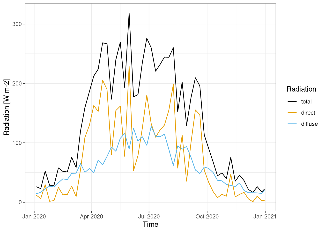
Figure 1.6: Direct and diffuse component of shortwave radiation over a year. Data is averaged weekly. Data from Hainich national park 2020.
Figure 1.7 shows a summer week, where it is possible to clearly see the difference between cloudy and sunny day. The 8th of July (first day) was cloudy with virtually no direct radiation, while the 13th of July was very sunny with almost all radiation direct.
shortwavedata%>%
  filter(week(Date)==28) %>%
  gather("type", "rad", Shortwave_incoming_W_m.2, direct, factor_key = T)  %>%
  ggplot(aes(x=Date, y=rad, color=type)) +
    geom_line() +
  scale_color_colorblind(labels=c("total", "direct")) +
  labs(y="Radiation [W m-2]", x="Time", col="Radiation")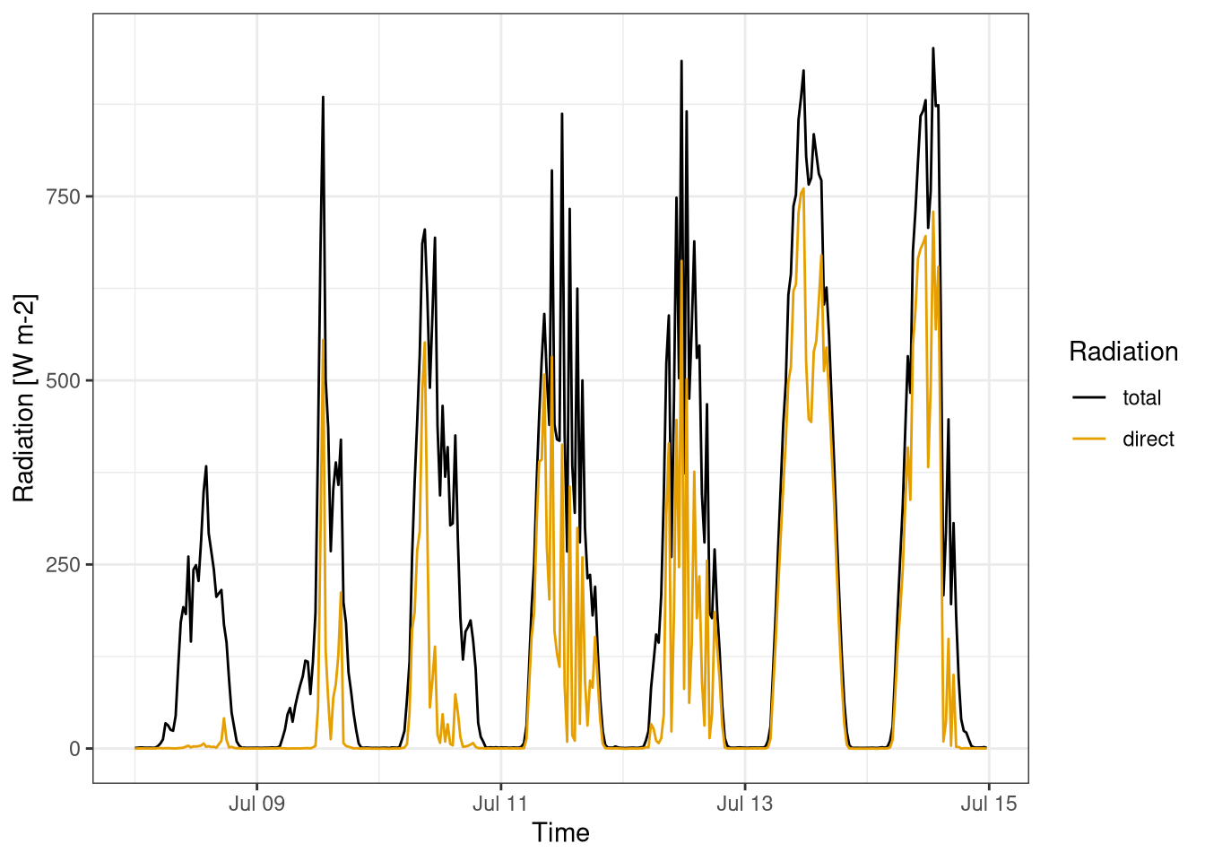
Figure 1.7: Total and direct component of shortwave radiation over a week. Data is averaged over 30 min. Data from Hainich national park second week July 2020.