4 Air humidity

4.1 Motivation

Air is a mixture of different gases and water vapour is a small fraction but still plays a crucial role for ecosystems.

The movement of water into the plant is driven by the transpiration, which happens as water leaving the plant from the leaf stomata. The features of this phenomenon are dependent on the amount of water present in the atmosphere, the lower the humidity the higher the stomata conductivity.

Water vapour is also important in the energy balance of ecosystems , as an significant fraction of the sun energy is converted is latent heat flux, or water evaporating goes from the surface.

4.2 Background

The behaviors of water in the air are complex and depending on the contest the are different variable used to measure the air humidity and connected parameters. They are:

• Actual vapor pressure [\(hPa\)]

The actual vapour pressure is the partial vapour pressure of water, which is the fraction of the total air pressure that is due to water moleculs. It is defined using the ideal gas law as following: It is one of the most common measurement of the air water content.

\[e_a = \rho_v R_v T\]

• Saturation vapour pressure [\(hPa\)]

The amount of water vapour that can be contained into the air is limited, the saturation vapour pressure is the water vapour pressure that a saturated air would have. It is strongly dependent on temperature increasing exponentially with incrase in temperatures. It can be estimated with the following formula:

\[e_s = 6.1078 e^{\frac{17.08085 T_a} {234.175°C + T_a}}\]

• Relative humidity [%]

The relative humidity is ratio between the actual vapur pressure and the saturation vapour pressure expressed in percentage. It is a common way of describing humidity.

• Dewpoint temperature [\(^{\circ} C\)]

The dew point temperature is the temperature when the water in the air would start condensing. This happens when the actual vapur pressure becomes equal to the saturation one. It can be estimated with the following formula:

\[T_d = \frac{(len(e_a) - ln(6.1708))\cdot234.17} {17.08085 - ln(e_a) + ln(6.1078)}\]

• Absolute humidity [\(Kg \quad m^{-3}\)]

The absolute humidity represent the actual mass of water present in a unit volume of air. It is defined as the density of water vapour:

\[\rho_v = \frac{e_a}{(R_v T)}\]

• Specific humidity [\(Kg / Kg\)]

The specific humidity (q) is the ratio between the density of water vapour of the density of moist air

\[q = \frac{e_a}{p-0.378 e_a}\]

• Mixing ratio [\(Kg / Kg\)]

The specific humidity (q) is the ratio between the density of water vapour of the density of dry air

\[q = \frac{e_a}{p-0.378 e_a}\]

• Vapor pressure deficit [\(hPa\)]

The vaopur pressure deficit is the difference between the saturation vapour pressure and the actual vapour pressure. It indicates which is the amount of water that can still be added in the atmosphere before reaching saturation.

• Equivalent temperature [\(^{\circ} C\)]

The equivalent temperature is the temperature that would be reached if the energy release by the condesation of all water is used to heat up the air mass. Therefore by definition it is always higher than the actual air temperature.

Can be estimated with the following formula:

\[T_{eq} = T_a + \frac{L_v}{C_p} m \approx T_a + 2.5 m \] where:

• \(L_v\) = \(2.5 10^6 J Kg^{-1}\) is the latent heat of vaporization
• \(C_p\) = \(1004.6 J Kg^{-1} K^{1}\) is the specific heat capacity of dry air
• \(m\) = mixing ratio in \(g / Kg\)
• \(T_a\) = air temperature in K

4.3 Sensors and measuring principle

There are numerous principles used to measure variable related to air humidity.

• Condensation. The condensation hygrometers measure the dew point temperature, when the moisture in the air start to condense.
  • Dew point mirror. There is a mirror that is cooled down to the dew point temperature. Small droplets on the mirror are then detected on the top of the mirror by a reflected LED light.
  • LiCL dew point hygrometer. The is a solution of LiCl, that is hygroscopic and conducts electricity only when wet. This is connected to an heating system is used to estimate the dew point temperature.
• Hygroscopic. The basic principle is the change of dimension due to the change in humidity. The most common sensor to use this principles is the Hair hygrometer, that uses a series of proerply treated horse hairs connected to a spring that change their size in relation to the relative humidity.
• Spectroscopric. Different gas absorbs certain infrared light at specific wavelengths and water vapour has it own characteristic asbosption bands. Infrared gas analyzer measure the amount of IR light that is absorbed by the air on some specific wavelenght and can use this information to estimate the number of water molecules. This sensors are used in Eddy Covariance setups and can provide high frequency and high accuracy measurements.
• Capacitative. Some material change their dialectic properties with the change of humidity, hence by measuring the change of capacity it is possible to estimate the air humidity. This sensors are fast, accurate and have long-term stability making them common.
• Psychrometric. The humidity is estimated by measuring the normal air temperature and the air temperature of a wet themometer. The wet thermometer will have a lower temperature as water evaporation substract energy. The amount of evaporation is related to the air humidity, hence by knowing the entity of the temperature reduction of the wet thermometer it is possible to calculate the air humidity. This principle is used by the Assmann and spinning Psychrometers, which allows to have an analong measurement of air humidity with a good accuracy.

4.4 Analysis

Using the field meaurement of relavitve humidity, air temperature and air pressure from the Hainich national park the following variables were calculated and used of the subsquent analysis.

1. Actual vapor pressure
2. Saturation vapor pressure
3. Dewpoint temperature
4. Absolute humidity
5. Specific humidity
6. Mixing ratio
7. Vapour pressure deficit
8. Equivalent temperature

hum <- read_csv(here("Data_lectures/4_air_humidity/04_Air_humidity_TA_RH_PA_NP_Hainich.csv"))
names(hum) <- c("datetime", "ta", "rh", "pa")

c2k <- function(c) c + 273.15
k2c <- function(k) k - 273.15

Rv <- 461.47 # J K -1 kg -1 ] - gas constant of water vapour
get_es <-  function(ta)  6.1078 * exp((17.08085 * ta) / (234.175 + ta))
get_td <- function(e_a) ((log(e_a) - log(6.1708)) * 234.17) / (17.08085 - log(e_a) + log(6.1078))
get_rh <- function(e_a, e_s) e_a/e_s * 100
rh2ea <- function(rh, e_s) rh/100 * e_s

# need to convert e_a from hPa to Pa and the temperature to degrees Kelvin
# convert the output in g/Kg 
get_abs_hum <- function(e_a, ta) (e_a * 100 / (Rv * c2k(ta)) ) * 1000

#here there is no need to convert to Pa
# because the pressures is present both at numerator and denominator
get_spec_hum <- function(e_a, p) 0.622 * e_a / (p - 0.378 * e_a) * 1000 # g/Kg
get_mix_ratio <- function(e_a, p) 0.622 * e_a / (p - e_a) * 1000 # g/Kg


get_p_def <- function(ea, es) es - ea
get_t_eq <- function(ta, mix_ratio) k2c(c2k(ta) + 2.5 * mix_ratio)

get_ea_dry <- function(es_wet, t_dry, t_wet, p){
  a <- (p * 1004.6) / (0.622 * 2.5061e6)
  return(es_wet - a * (t_dry - t_wet))
}

# utility func for plotting
remove_x_axis <- function() theme(
    axis.text.x = element_blank(),
    axis.title.x = element_blank(),
    axis.ticks.x = element_blank()
  )

# add all the variables to the humidity dataframe
hum <- mutate(hum,
    es = get_es(ta),
    ea = rh2ea(rh, es),
    td = get_td(ea),
    abs_hum = get_abs_hum(ea, ta),
    spec_hum = get_spec_hum(ea, pa),
    mix_ratio = get_mix_ratio(ea, pa),
    p_def = get_p_def(ea, es),
    t_eq = get_t_eq(ta, mix_ratio)
  )

hum_d <- hum %>%
  group_by(week=yday(datetime)) %>%
  summarize_all(mean, na.rm=T)

hum_w <- hum %>%
  group_by(week=week(datetime)) %>%
  summarize_all(mean, na.rm=T)

4.4.1 Actual and saturation vapour pressure

The saturation vapour pressure and the actual vapour pressure are compared during one year (Figure 4.1) and during one week time period (Figure 4.2).

hum_d %>%
  gather("type", "val", es, ea, factor_key = T) %>%
  ggplot(aes(datetime, val, colour=type))+
    geom_line()+
  labs(x="Time", y="Vapour pressure [hPa]", colour="Vapur pressure") +
  scale_color_colorblind(labels=c("saturation", "actual")) +
  theme(legend.position = "bottom")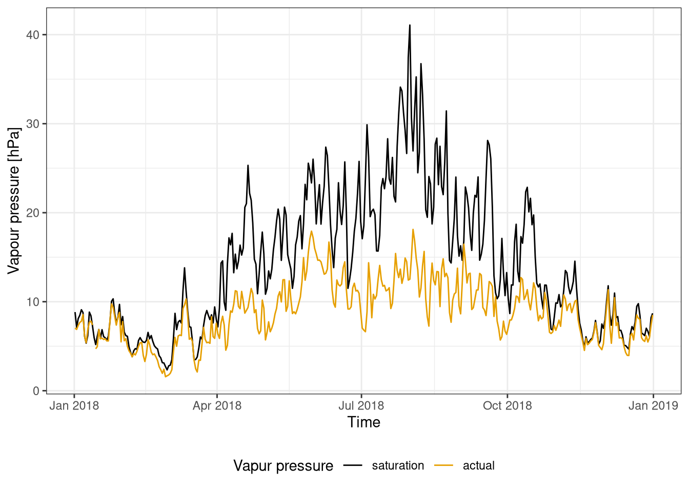

Figure 4.1: Comparison between saturation vapour pressure and actual vapour pressure for one year. Data averaged on a day. Data from Hainich national park 2018.

hum %>%
  filter(week(datetime) ==1) %>%
  gather("type", "val", es, ea, factor_key = T) %>%
  ggplot(aes(datetime, val, colour=type))+
    geom_line()+
    labs(x="Time", y="Vapour pressure [hPa]", colour="Vapur pressure") +
    scale_color_colorblind(labels=c("saturation", "actual"))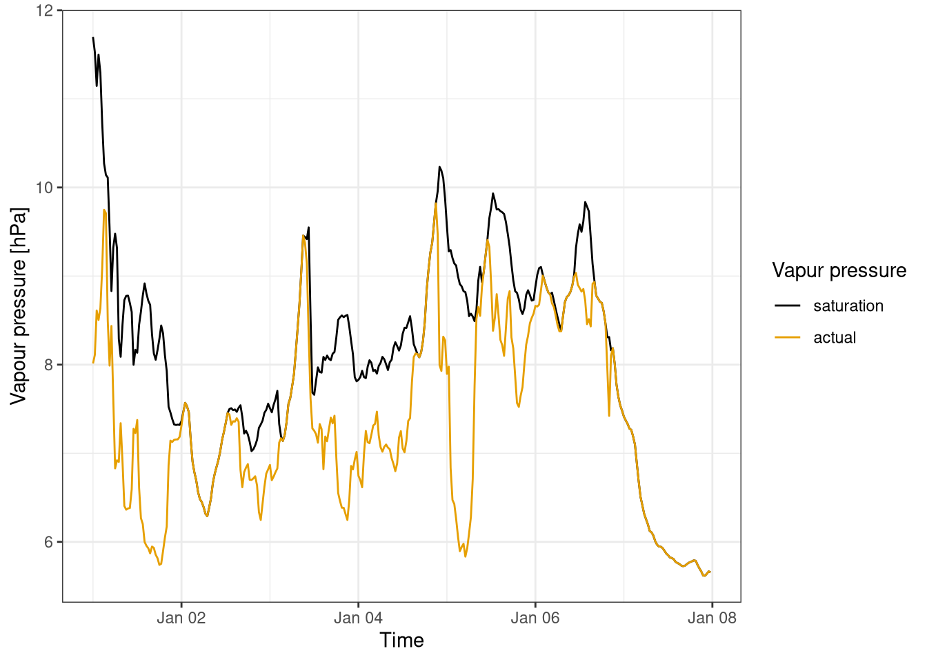

Figure 4.2: Comparison between saturation vapour pressure and actual vapour pressure for the first week of the year. Data averaged over 30 minutes. Data from Hainich national park 2018.

During the year the saturation water vapour ranges from around 5 hPa in the winter to more than 40 hPa in August. There is a clear yearly cycle that is directly connected to the change of air temperature.

The variation in actual vapour pressure are much smaller, but still show a seasonal pattern.

During the summer there is the biggest different between the actual and the saturation vapour pressure, due to the the high saturation vapour pressure but relatively limited water availability. Conversely during winter the saturation vapour pressure is much smaller and the water availability higher resulting in a small pressure deficit.

4.4.2 Air and dew point temperature

The relative humidity and the air and dew point temperature are compared (Figure 4.3).

p_td <- hum_d %>%
  gather("type", "val", ta, td) %>%
  ggplot(aes(datetime, val, colour=type))+
    geom_line()+
  labs(x="Datetime", y="Temperature [°C]", colour="Temperature") +
  scale_color_colorblind(labels=c("air", "dew point")) +
  remove_x_axis()

p_rh <- ggplot(hum_d, aes(datetime, rh))+
    geom_area() +
  geom_hline(yintercept = 100, linetype="dashed", size=.2) +
  labs(y="Rel. humidity [%]", x="Time")

p_td / p_rh +
  plot_layout(heights = c(4, 2)) +
  plot_annotation(tag_levels = "a")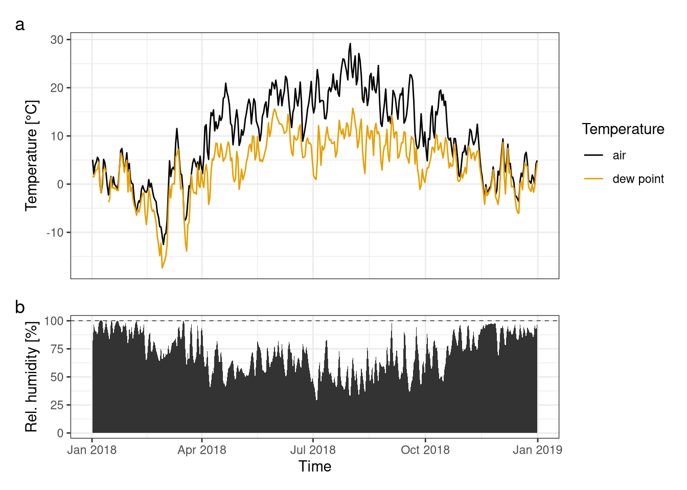

Figure 4.3: Comparison of air temperature with dew point temperature (fig. a), showed in relation with the relative humidity (fig. b). Data averaged over one day. Data from Hainich national park 2018.

With the analysis of the graphs, a direct relationship between a lower amount of relative humidity during summer and wider difference between the graphs of Tair and Tdewpoint can be concluded. This means, that the temperature of air reaches its peak in summer due to less relative humidity in air, while at the beginning and end of the year more similarities can be seen.

4.4.3 Absolute humidity

The absolute humidity is largest during the summer compared to winter (Figure 4.4). This may seem counterintuitive as during winter the relative humidity is much higher than during summer, however the amount of water that can be hold in the air during summer is much higher than during winter. In fact the is a strong relation with temperature as can be seen in the last week of March where there is a sudden drop in the the absolute humidity.

hum_d %>%
  ggplot(aes(datetime, abs_hum))+
    geom_line() +
  labs(x="Datetime", y="Absolute humidity [g/kg]")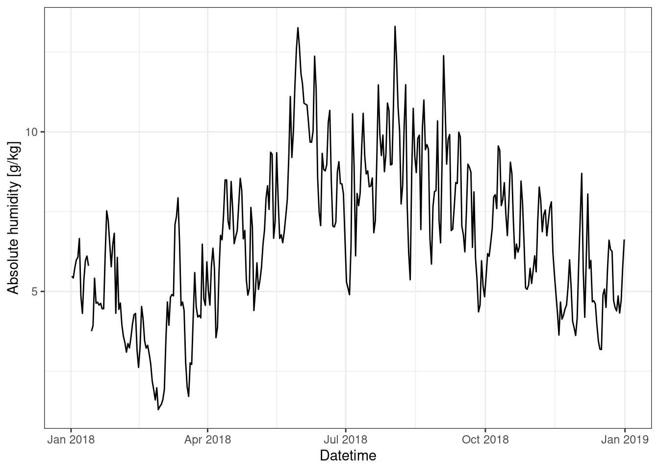

Figure 4.4: Absolute humidity over the year. Data averaged over one day. Data from Hainich national park 2018.

4.4.4 Mixing ratio and specific humidity

The mixing ratio and the specific are very similar (Figure 4.5). The only different between them is that the first if the density of water is calculated over dry air in the former and moist in the latter. It is possible to see that with higher values of mixing ratio, and therefore water content, the difference between the two variable is bigger to to the bigger difference in density between wet and dry air.

hum %>%
  filter(week(datetime) ==30) %>%
  gather("type", "val", spec_hum, mix_ratio) %>%
  ggplot(aes(datetime, val, colour=type))+
    geom_line() +
    labs(y="Water content [Kg/Kg]", colour="", x="Time") +
    scale_color_colorblind(labels=c("Mixing ratio", "Specific humidity"))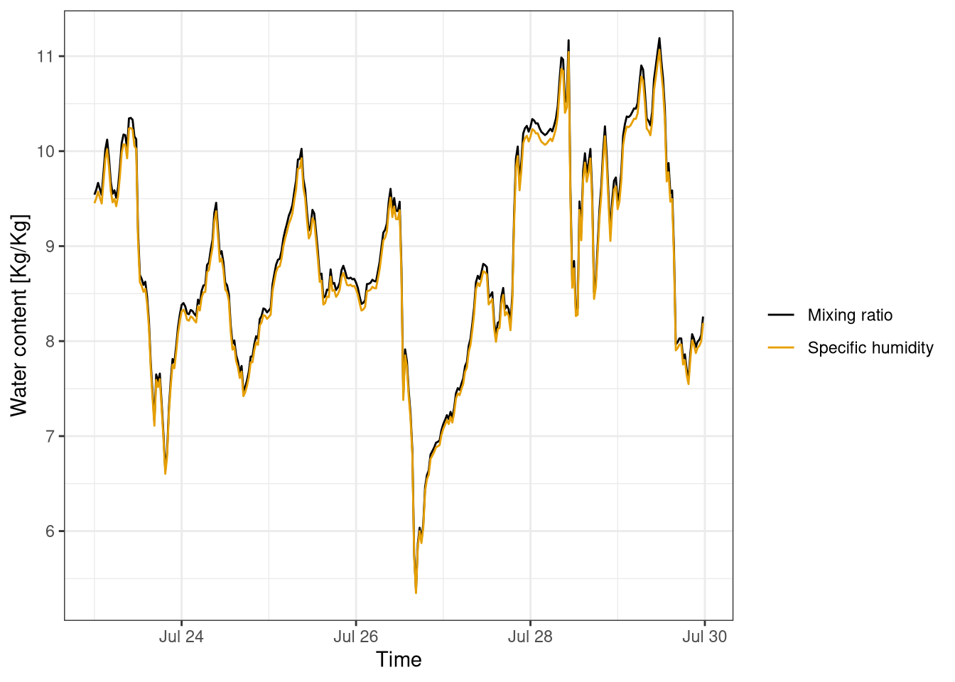

Figure 4.5: Comparison of mixing ratio and specific humidity. Data averaged at 30 minutes from last week of July 2018. Data from Hainich national park.

4.4.5 Vapour pressure deficit

The vapour pressure deficit has a yearly cycle (Figure 4.6), it is almost zero during the winter and reaches its maximum during the summer.

hum_d %>%
   ggplot(aes(datetime, p_def)) +
   geom_line() +
   labs(y="Pressure deficit [hPa]", x="Time")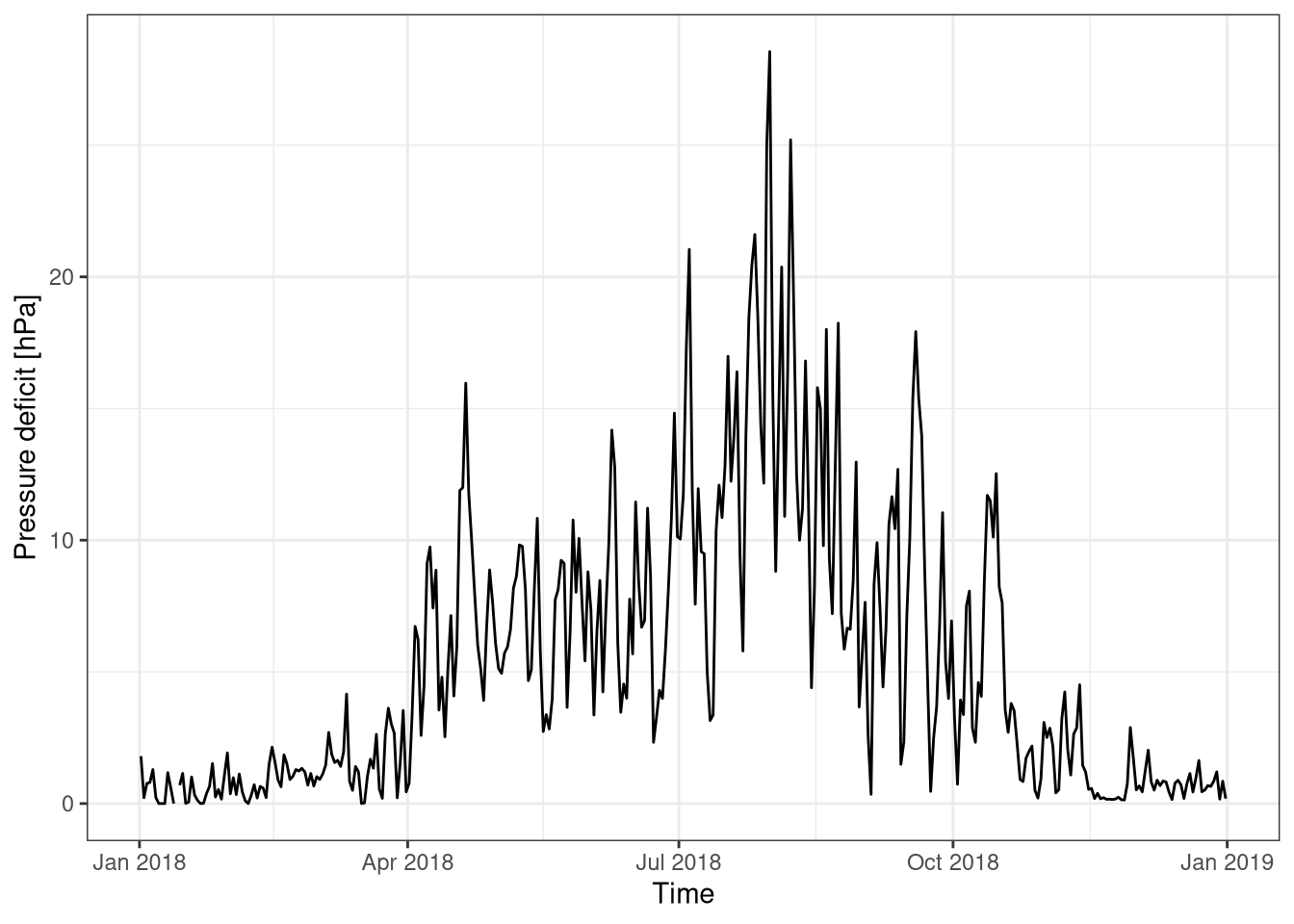

Figure 4.6: Vapur pressure deficit over the year. Data averaged over one day. Data from Hainich national park 2018.

The vapour pressure deficit has also a daily cycle (Figure 4.7), with higher values during the afternoon where the temperature is still high but the water reserves have been depleted during the day. It then reaches a minimum in the early hours of the morning, mainly due to the low temperatures.

hum %>%
  filter(week(datetime) == 30) %>% 
   ggplot(aes(datetime, p_def)) +
   geom_line() +
   labs(y="Pressure deficit [hPa]", x="Time")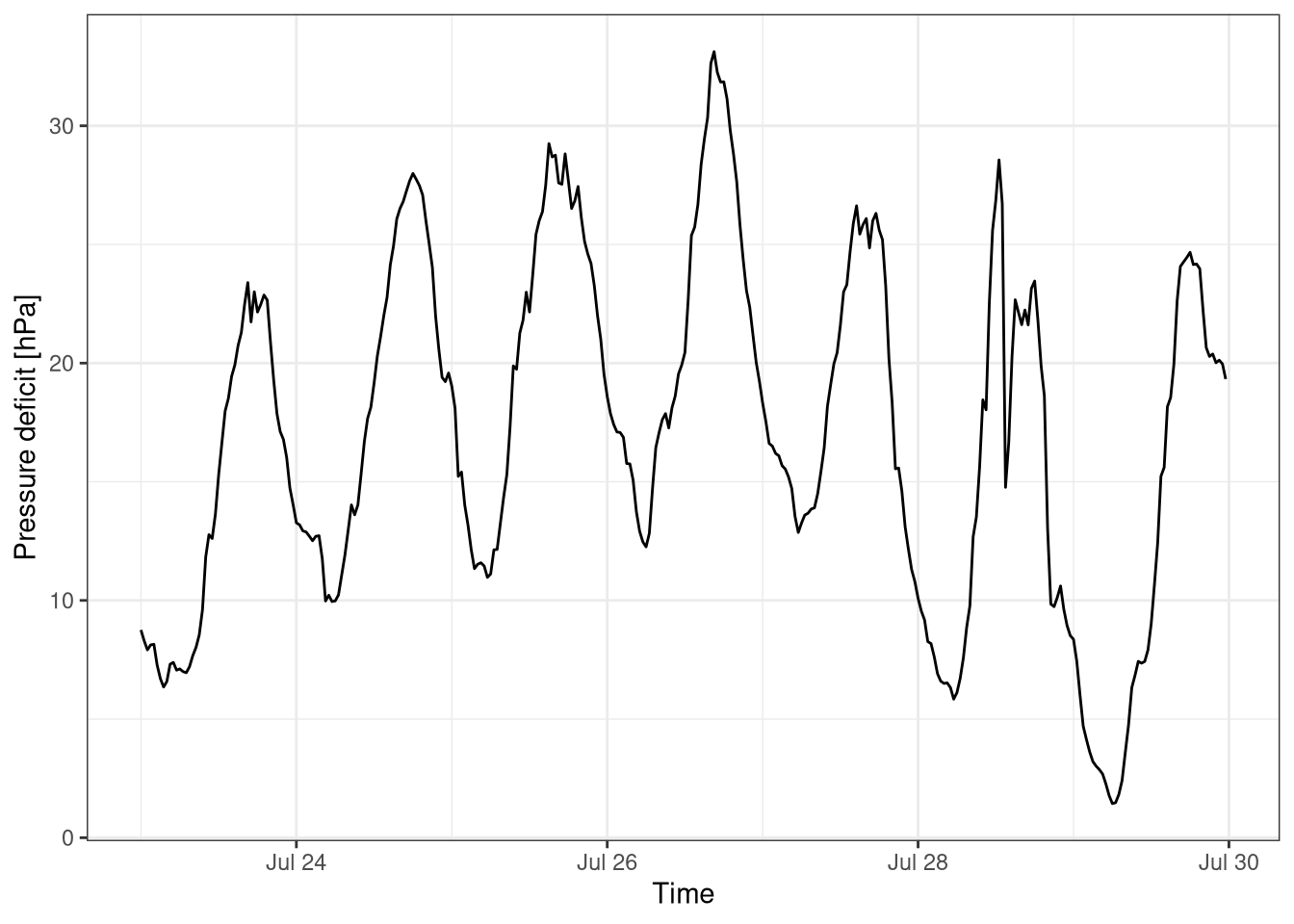

Figure 4.7: Vapur pressure deficit over one week. Data averaged over 30 mins. Data from Hainich national park last week july 2018.

4.4.6 Equivalent temperature

The equivalent temperature is of course strongly dependent on the base air temperature, but the difference is bigger when the absolute humidity is higher, hence it has a yearly cycle (Figure 4.8). During the summer the equivalent temperature is roughly the double of the air temperature.

hum_d %>%
  gather("type", "val", t_eq, ta, factor_key = T) %>%
  ggplot(aes(datetime, val, colour=type))+
    geom_line() +
    scale_color_colorblind(labels = c("Equivalent", "Air")) +
    labs(y="Temperature [°C]", x="Time", colour="Temperature")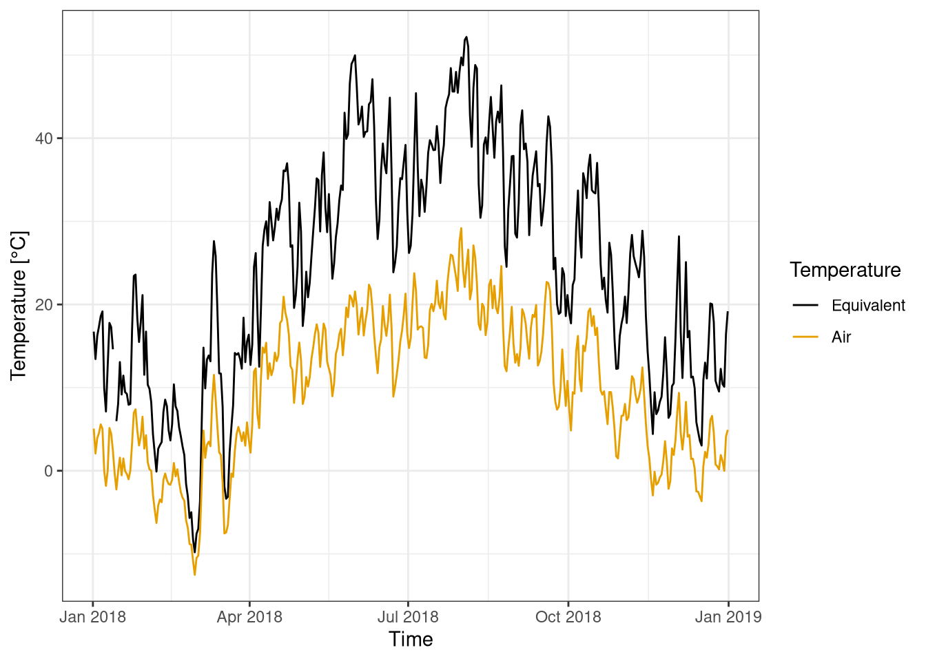

Figure 4.8: Equivalent temperature compared to air temperature. Data averaged over one day. Data from Hainich national park 2018.

4.4.7 Field humidity measurements

The humidity has been measured in the field using two different psychrometer, an assmann and an spinning one. The measures of the the instruments are compared in table 4.1. The two measures are comparable but show a significant difference (~20 % in relative humidity). This is incongruence is probably due to inaccuracies in the measurement and possibly different conditions between the measures. Moreover the thermometers of the spinning psychrometer are not protected from the direct sunlight which can compromise the reading, in fact the dry temperature is higher and the wet temperature is lower in the spinning psychrometer.

spin <- tibble(
  t_dry = 16,
  t_wet = 10.8,
  p = 977.2
)

spin <- spin %>%
  mutate(
    es_wet = get_es(t_wet),
    es = get_es(t_dry), 
    ea = get_ea_dry(es_wet, t_dry, t_wet, p),
    td = get_td(ea),
    rh = get_rh(ea, es),
    abs_hum = get_abs_hum(ea, t_dry),
    spec_hum = get_spec_hum(ea, p),
    mix_ratio = get_mix_ratio(ea, p),
    p_def = get_p_def(ea, es),
    t_eq = get_t_eq(t_dry, mix_ratio)
    
  )

assman1 <- tibble(
  t_dry = 15.4,
  t_wet = 11.8,
  p = 977.2
) %>%
  mutate(
    es_wet = get_es(t_wet),
    es = get_es(t_dry), 
    ea = get_ea_dry(es_wet, t_dry, t_wet, p),
    td = get_td(ea),
    rh = get_rh(ea, es),
    abs_hum = get_abs_hum(ea, t_dry),
    spec_hum = get_spec_hum(ea, p),
    mix_ratio = get_mix_ratio(ea, p),
    p_def = get_p_def(ea, es),
    t_eq = get_t_eq(t_dry, mix_ratio)
    
  )

spin %>% 
  bind_rows(assman1) %>% 
  t() %>% 
  kableExtra::kbl(col.names = c("Spinning", "Assmann"), digits = 1, caption = "Comparioson of measurement between spinning and assman psychrometer", booktabs=T) %>% 
  kableExtra::kable_styling(latex_options = "hold_position")

Table 4.1: Comparioson of measurement between spinning and assman psychrometer

	Spinning	Assmann
t_dry	16.0	15.4
t_wet	10.8	11.8
p	977.2	977.2
es_wet	13.0	13.9
es	18.2	17.5
ea	9.7	11.6
td	6.4	9.0
rh	53.2	66.2
abs_hum	7.3	8.7
spec_hum	6.2	7.4
mix_ratio	6.2	7.5
p_def	8.5	5.9
t_eq	31.6	34.1