2 Longwave radiation

2.1 Motivation

All bodies with a temperature above the absolute zero emit electromagnetic radiation. The wavelength and intensity of this radiation depends on the temperature of the body. Within the temperature range of the earth surface, the emitted radiation has a wavelength between 3 and 100 mm and it is defined as longwave.

Emitting longwave radiation is the only way for the plant to cool itself down, making it a crucial component in the overall energy balance of the earth. In fact climate change is caused by green house emissions, which capture part of the longwave radiation emitted by the planet surface and then re-emit in back towards the Earth. This results in a bigger amount of radiation reaching the earth surface, hence increasing its temperature (Harries 1996).

Longwave is a constantly present in terrestrial ecosystem for all the day. Energy loss in form of longwave radiation can have a substantial impact on the surface temperature, especially during night.

2.2 Background

Longwave radiation is electromagnetic radiation with a wavelength between 3 and 100 mm, hence it falls into the Infrared section of the spectrum.

The overall amount of radiation emitted by a body depends on its temperature following the Stefan-Boltzmann law (Bonan 2019).

\[E = \varepsilon \sigma T^4\] Where:

• \(E\) is the radiation intensity in \(W/m^2\)
• \(\varepsilon\) an adimensional coefficient that represents the emissivity of the body. This depends on the material, a perfect black body has a \(\varepsilon\) of \(1\), while other materials have a lower emissivity
• \(\sigma\) is the Steffan-Boltzman constant \(5.67 \times 10^{-8} W m^{-2} K^{-4}\)
• \(T\) is the body temperature in \(K\)

As a consequence of Stefan-Boltzmann law the amount of longwave radation emitted by ecosystems depents on their temperature.

The incoming longwave radiation depends on the temperature of the sky and it is partly absorbed by the ecosystems and partly reflected (Stephens et al. 2012) according to the following formula:

\[L_{w, relf} = (1-\varepsilon)L_{w, in}\]

The amount of longwave radiation incoming depends on the temperature of the sky, hence in cloudy days there is an higher incoming longwave radiation compared to sunny days. This phenomenon is particularly important at nights, where the longwave balance is a major driver of the overall temperature.

The net longwave radiation is summarized by this equation:

\[L_{w, net} = L_{w, in} - L_{w, refl} - L_{w, emit}= \varepsilon(\sigma\varepsilon_{sky} T^4_{sky}) - \sigma\varepsilon T^4\] The overall net radiation includes also the shortwave component:

\[R_{w, net} = S_{w, in} - S_{w, out} + L_{w, in} - L_{w, out}\]

2.3 Sensors and measuring principle

The longwave radiation is estimated by measuring the change of temperature of a body exposed to the radiation. Compared to shortwave radiation the measured data required further processing as the sensor itself emits longwave radiation, hence there is the need include it the final measurement.

\[ L_{tot}= L_{net} + \sigma T_{sensor}^4 \]

Moreover the longwave sensors need to filter the incoming radiation to avoid measuring the shortwave component, therefore they usually have a filter that allows only infrared radiation between of 4.5 and 40 micrometers. This principle is used by pyrgeometers .

Longwave radiation can also be measured together with shortwave by net radiation sensors that don’t filter the incoming radiation based on wavelength.

Finally pyrometer, or infrared thermometers, measure the temperature of a body using the emitted longwave radiation. The use of the longwave radiation permits to have high frequency measures and more importantly to measure the temperature from a distance. However the emissivity of the body needs to be estimated to correctly

2.4 Analysis

rad <- read_csv(here("Data_lectures/2_Longwave_radiation/LW_SW_TSoil_BotGarten.csv"))
names(rad) <- c("datetime", "t_sens", "sw_in", "sw_out", "lw_in_sens", "lw_out_sens", "t_soil")

# Utlitity funcs
sigma <- 5.67e-8 

lw2temp <- function(lw) (lw/ sigma)^(1/4)
temp2lw <- function(temp)  return (sigma * temp^4)

c2k <- function(c) c + 273.15
k2c <- function(k) k - 273.15

#calculate from input data the real lw and the soil/surface temperature
rad <- rad %>%
  drop_na() %>%
  mutate(
    lw_sens = temp2lw(c2k(t_sens)),
    lw_in = lw_in_sens + lw_sens,
    lw_out = lw_out_sens + lw_sens,
    t_sky = lw2temp(lw_in) %>% k2c,
    t_surface = lw2temp(lw_out) %>% k2c,
    net_rad = lw_in - lw_out + sw_in - sw_out,
    net_sw = sw_in - sw_out,
    net_lw = lw_in - lw_out
  )

# for making aggregation easier we are going to consider data only for one calendar year
rad <- rad %>%
  filter(datetime < as_datetime("2020-12-31"))

# weekly average data
rad_w <- rad %>% 
  as_tsibble(index = datetime) %>%
  index_by(week = ~ yearweek(.)) %>%
  summarise_all(mean, na.rm = TRUE)

# daily average data
rad_d <- rad %>%
  mutate(yday = yday(datetime)) %>%
  group_by(yday) %>%
  summarize_all(mean, na.rm = TRUE)

2.4.1 Surface and Sky temperature

The surface and the sky temperature are plotted for one year using a weekly (Figure 2.1) and daily aggregation (Figure 2.2).

The sky temperatures is always lower than the surface one. The surface temperature ranges from -2 C to 25 C, while the sky temperature has a bigger range from -23 C to 17 C. The temperature of the sky mainly depends on the cloud cover and the temperature of the air.

During the last week of march there is biggest different in temperature, with the sky temperature plummeting to -20 °C, while the surface temperature remains above 0 °C. This is probably due to snow cover that insulates the surface from the cold air. For the rest of the year the temperature difference is relatively constant.

rad_w %>%
  gather(key="type", value="temp", t_surface, t_sky, factor_key = T) %>%
ggplot(aes(x=datetime, y=temp, colour=type)) +
  geom_line() +
  scale_color_colorblind() +
  labs( y="Temperature [°C]", x="Time")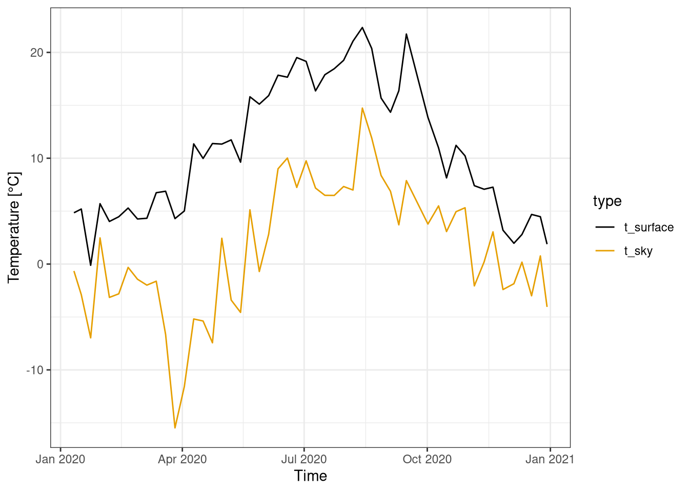

Figure 2.1: Weekly average of sky and surface temperatures over one year. Data from botanical garden 2020.

rad_d %>%
  gather(key="type", value="temp", t_surface, t_sky, factor_key = T) %>%
ggplot(aes(x=datetime, y=temp, colour=type)) +
  geom_line()  +
  scale_color_colorblind() +
  labs(y="Temperature [°C]", x="Time")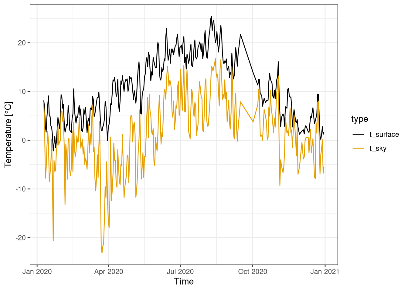

Figure 2.2: Daily average of sky and surface temperatures over one year. Data from botanical garden 2020.

The difference between the sky at the surface temperature is also analyzed using high frequency data (10 minutes) for a month (Figure 2.3) and a week (Figure 2.4).

The surface temperature has a clear day cycle and in the month of July for the majority of the time oscillates in the 10°C - 30°C range.

On the other hand the sky temperature has no daily cycle, but over the month has still important variations from -5°C to 20 °C.

Moreover, it can be clearly seen how during cloudy days (eg. 9th of July) there is a high sky temperature, but a low surface temperature. Conversely, on sunny days (eg. 7th of July) the surface temperature is higher, but the sky temperature is low.

rad %>%
  filter( month(datetime) == 7 ) %>%
  gather(key="type", value="temp", t_surface, t_sky, factor_key = T) %>%
ggplot(aes(x=datetime, y=temp, colour=type)) +
  geom_line()  +
  scale_color_colorblind() +
  labs(y="Temperature [°C]", x="Time", col="") +
  theme(legend.position = "bottom")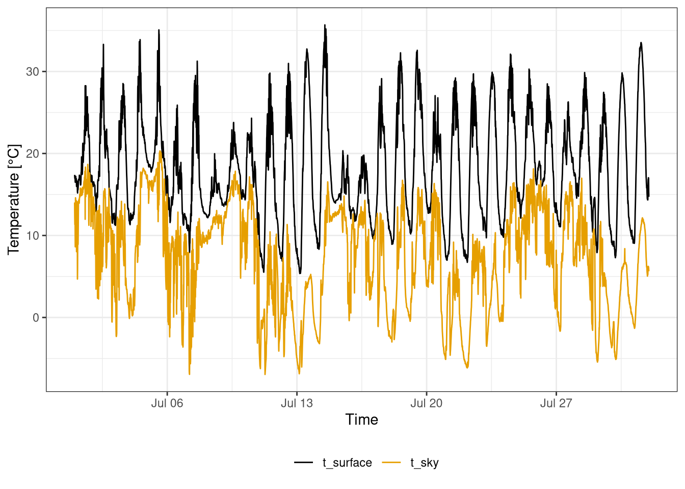

Figure 2.3: Sky and surface temperatures during July 2020. Data frequency 10 minutes. Data from botanical garden.

filter(rad, between(datetime, as_datetime("2020-07-03"), as_datetime("2020-07-12"))) %>%
  gather(key="type", value="temp", t_surface, t_sky, factor_key = T) %>%
ggplot(aes(x=datetime, y=temp, colour=type)) +
  geom_line()  +
  scale_color_colorblind() +
  labs(y="Temperature [°C]", x="Time", col="") +
  theme(legend.position = "bottom")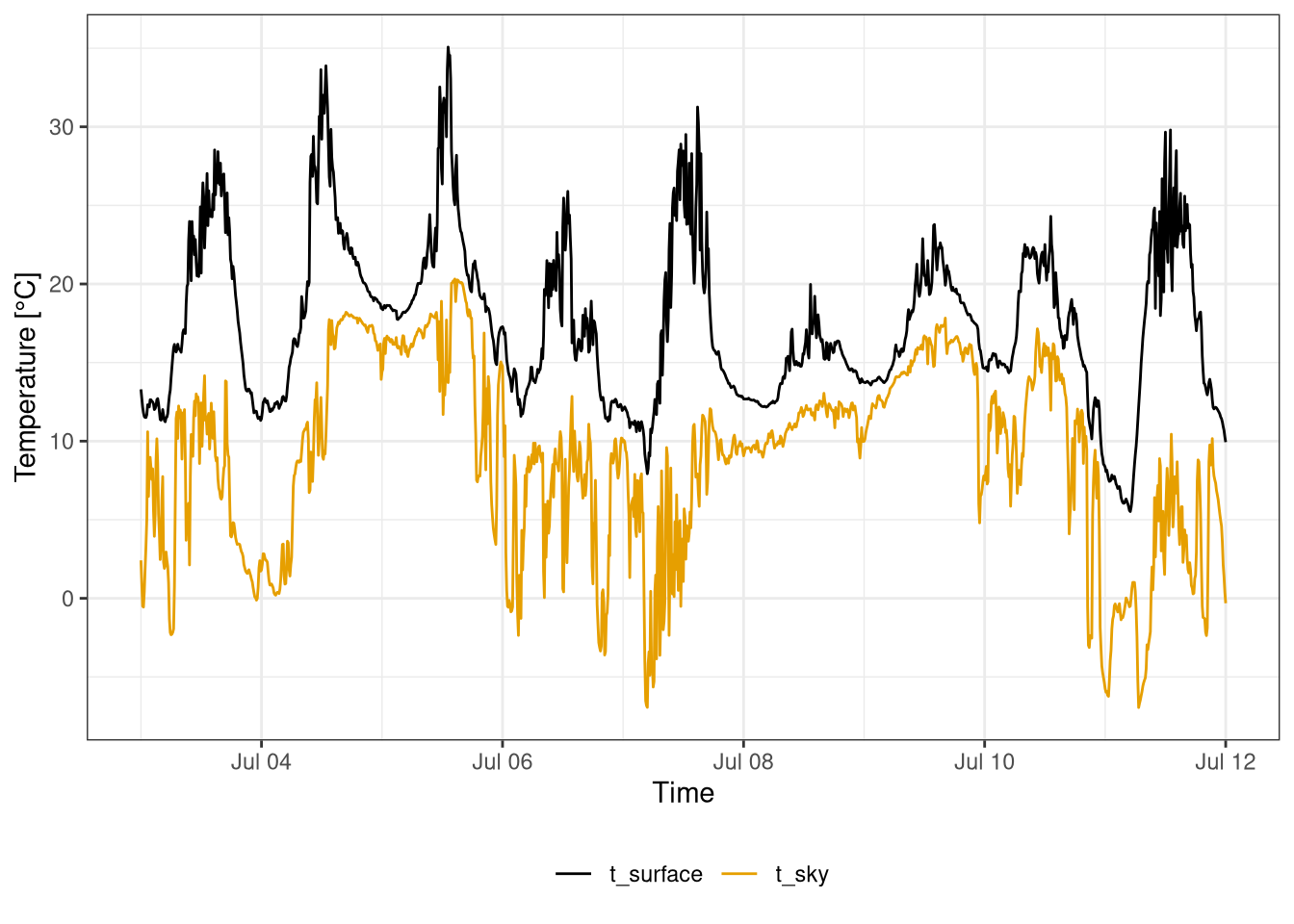

Figure 2.4: Sky and surface temperatures during first weeek of July 2020. Data frequency 10 minutes. Data from botanical garden.

2.4.2 Net radiation

The longwave and shortwave components are merged to calculate the overall net radiation for one year in figure 2.5.

The net radiation has a yearly cycle. During the summer it has a relatively constant value at around \(100 W/m^2\), then it decrease and reach slightly negative values in January. The biggest driver of this yearly cycle is the incoming shortwave radiation, which during summer is much higher than in winter. The radiation from the sun has smooth variations, while the variation on the incoming shortwave during the summer can be explained by the different amount of cloud cover. You would expect a clearer peak of the shortwave radiation during the summer, Moreover the net radiation has an high peak in mid late September. This behavior can probably be explained by different amount of cloud cover.

The outgoing shortwave is the component with the smallest absolute value, it also has a yearly cycle being virtually zero in January but quickly reaching the max value during the spring and then remaining quite flat. Regarding the longwave the outgoing radiation is always bigger than the incoming, due to the higher temperature of the surface compared to the sky. The longwave components have a much smaller change during the year.

There is a notable low peak of incoming longwave in the last week of march, that is probably explained by clear skies but still low air temperature.

rad_w %>%
  gather(key="type", value="radiation", lw_out, lw_in, sw_in, sw_out, net_rad,
         factor_key = T) %>%
ggplot() +
  geom_line(aes(x=datetime, y=radiation, colour=type)) +
  scale_color_colorblind() +
  labs(y="Radiation [W m-2]",
       x="Time", colour="Radiation")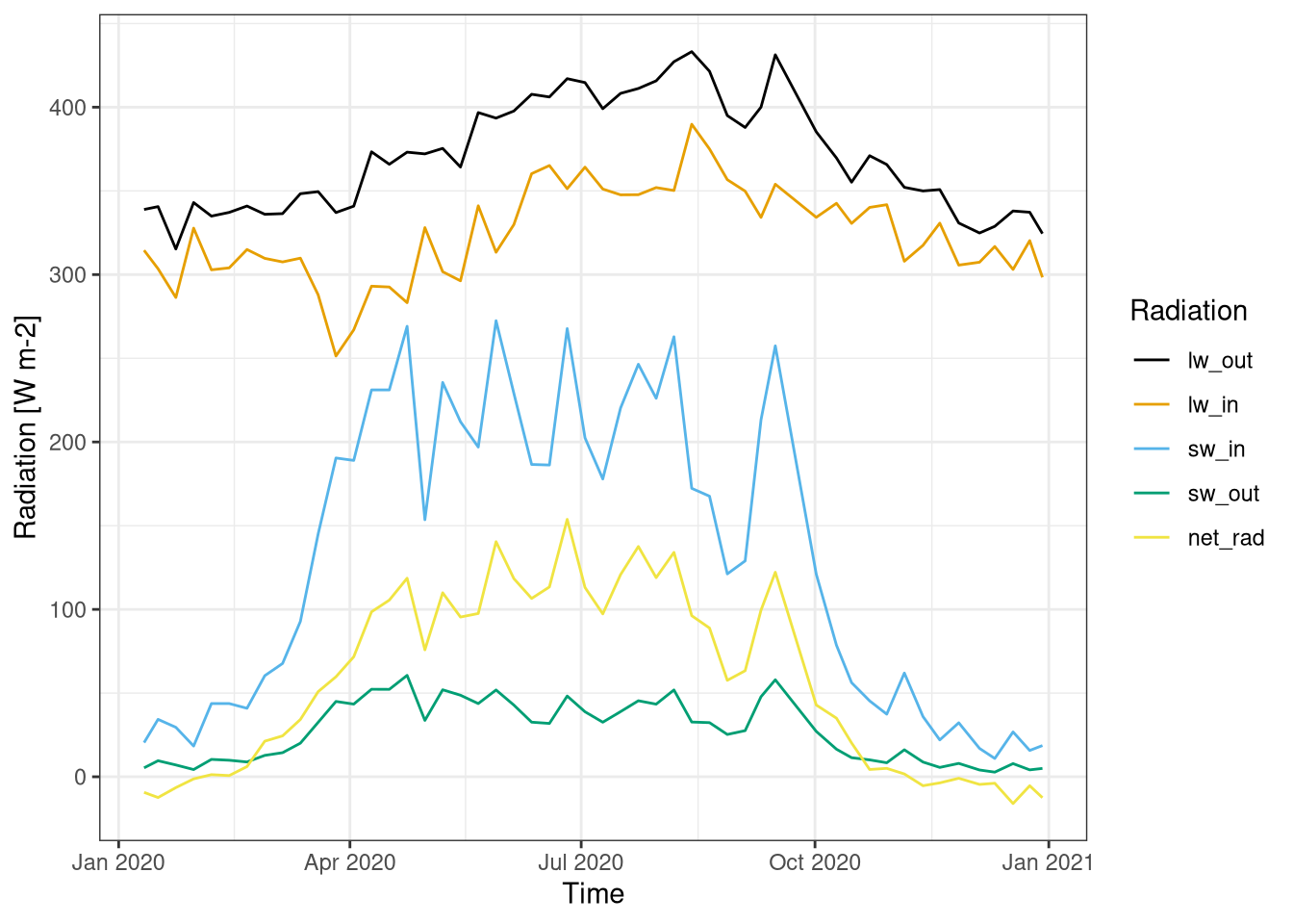 

Figure 2.5: Net radiation over the year. The four components of the radiation (shortwave incoming, shortwave outgoing, longwave incoming, longwave outgoing) are also showed. Data averaged over a week. Data from botanical garden 2020.

2.4.3 Change emissity in the sensor

In the field activity we tried to measure the temperature of the surface by using different emissivity settings in the sensor and see how that could influence the readings. However, there have been some issues with the sensor, so the data has been generated using the formula from the theory

In this virtual experiment the real temperature is set to 19 °C and the emissivity is changed, resulting in different temperature estimates.

t_0 <- 19 # temperature with emissivity 1
rad_0 <- c2k(t_0) %>% temp2lw # connected radiation 

temps <- tibble(
  em = seq(1, .1, -.05),
  t = (rad_0 / (em * sigma))^(1/4)  %>% k2c
) 

ggplot(temps, aes(em, t)) +
  geom_line() +
  scale_x_reverse() +
  labs(x="Emissivity", y="Temperature [°C]")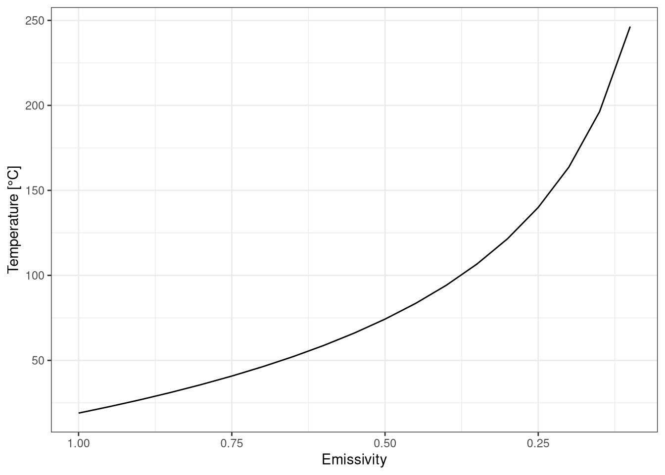

Figure 2.6: Estimanted temperature measured by infrared themometer for different emissivity. Temperature at emissivity 1 is 19 °C

It can be seen that the emissivity has a big influence on the temperature estimate. The emissivity of material can change drastically from \(0.03\) for aluminum foil to \(0.97\) for ice. This clearly shoes the importance of a correct estimation of the emissivity for temperature measurements.