9 Evapotranspiration

9.1 Motivation

The evapotranspiration (ET) is an important variable for ecosystems, as it represents the amount of water that is evaporating. This is a good indication of the amount of photosyntetic activity and by comparing it the potential ET water stress of ecosystems can be estimated.

Evaporanspiration is important to hold the global and continental scale hydrologic cycle. Evapotranspiration is influenced by a combination of factors; the increase of temperature, decrease of bulk canopy due to higher CO2 emissions and large scale land use change. (Likens and 1935- 2009)

9.2 Background

The ET is the actual amount of water that evaporates. In contrast the potential ET is the amount of water that would evaporate if there would be unlimited water available in the soil (Labedzki 2011).

The difference between the ET and the potential ET indicates the water stress of an ecosystem.

The measurement unit for ET is mm. The ET is often the ET on a daily basis.

The ET is measured in the field using different instruments, while the potential ET can be either measured or estimated using other enviromental variables.

In particular the Penman-Monteith is the most precise way to estimate the ET. It takes into account the energy available from the sun and the speed at which the water can evaporate, that depends on temperature, air humidity and wind.

\[{LE=\frac{s (R_n-G) + \rho_a c_p \left( e_s - e_a \right) / r_a } {s + \gamma \left ( 1 + r_a / r_s \right)}}\]

where:

• \(S\) Slope of saturation vapor pressure (kPa / K)
• \(R\) N Net radiation (W m -2 )
• \(G\) Ground heat flux (W m -2 )
• \(\rho\) Air density (kg m -3 )
• \(C_p\) Specific heat capacity at constant pressure (J kg -1 K -1 )
• \(e_s\) Saturation vapor pressure (kPa)
• \(e_a\) Actual vapor pressure (kPa)
• \(\gamma\) Psychrometric constant (kPa K -1 )
• \(r_s\) Stomata resistance (s m -1 )
• \(r_a\) Aerodynamic resistance (s m -1 )

A useful aproximation of the Penman-Monteith equation is the Priestley-Taylor formula which requires less meteorolical data

\[ PET \approx 1.26 \frac{s}{s+\gamma} \left(R_N - G \right) \] where:

• PET is the daily evapotranspiration
• s is the saturation vapour pressure (\(kPa/K\))
• \(R_N\) is the net radiation in \(MJ / m^2 d\)
• \(G\) is the soil heat flux in \(MJ / m^2 d\)

9.3 Sensors and measuring principle

There are many different ways to measure evapotranspiration,some are more accessible than others and depending the scenario some of them might be more suitable than others. The measurement of evapotranspiration claims quantitative data, and this data can be measure by water evaporation and the energy flux between soil and atmosphere. Rana and Kater (2000), describes the different ways to measure evapotranspiration based on hydrological, micrometeorological, plant physiology and analytic approaches. The first one includes: soil water balance and weighing lysimeters, the second one, energy balance and Bowen ration, aerodynamic method and eddy covariance. Plant physiology approach is based on sap flow method or chambers system. Last one, analytical approach are based on Penman-Montheith model. After this one, empirical approach can also be taken into account, such as process based on crop coefficient approach and soil water balance modeling (Rana and Katerji 2000).

Some of the most frequently measurements applied to evapotranspiration and that we have seeing in class are:

• Evaporation pan: a circle panel where precipitation is accumulated and then, with the help of a measuring bucket and based on a scale, water loss can be measured by the difference between the potential evapotranspiration of 2 days. Some of the errors are related to the expansion of water, wrong reading, limited recording for a volume of water and the possibility of the oasis effect to occur.

• Piché evaporimeter: is a type of atometer applied in the measurement rate of evaporation from a wet disc with absorbent paper. Results are dependent on wind speed that goes through the disc, as well as the wet bulb saturation deficit. The rate of evaporation is usually expressed as the volume of water evaporated per unit area in unit time.

• Weighing lysimeter: they allow the mass or volumetric soil water content variation to be measured by weighing the lysimeter and determining its change of mass over time. They can measure the net infiltration from precipitation or irrigation systems and the quantity of net evaporation between different wetting events (Meissner, Rupp, and Haselow 2020).

Bowen ratio energy balance method: also known as BREB method has been widely used to quantify water balance. It estimates the latent heat flux from a surface using measurements of air temperature and humidity gradients, net radiation and soil heat flux. In comparison with other methods such as eddy covariance or weighting lysimeters, is an indirect method (Todd, Evett, and Howell 2000). Some advantages are that it does not require information about aerodynamic characteristics of zone of interest, it integrates latent hear fluxes over a wide areas and gives an estimation of these flux in short time period intervals (e.g. less than half hour).

9.4 Analysis

9.4.1 Potential evapotranspiration

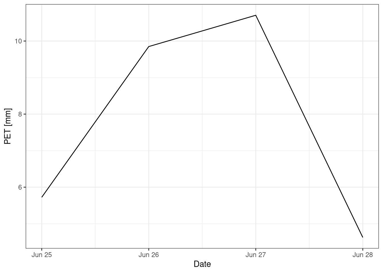
During the four days of measurement the potential ET has been estimated using the Priestley-Taylor (Figure 9.1). The daily potential ET varies a significantly during the 4 days, ranging from 6mm to almost 12 mm. This reflects the change in the weather conditions, as the day 1 and 4 were cloudy and colder.

library(tidyverse)
library(lubridate)
library(scales)
theme_set(theme_bw())

et <- "Data_lectures/09_Turbulent_fluxes_I_ET/ET_data_forst_botanical_garden.csv" %>% 
  here::here() %>% 
  read_csv(locale = locale(decimal_mark = ",")) %>% 
  rename(loc_id = replicates)
meteo <- 
  "Data_lectures/09_Turbulent_fluxes_I_ET/MeteoData_BotanicalGarden.csv" %>% 
  here::here() %>% 
  read_csv()

#' Potential evapotranspiration using Priestley-Taylor equation
calc_pet <- function(T_air, Rn, G){
  g <- 0.067 # kPa K -1
  s <- ( 4098 * (0.6108 * exp((17.27 * T_air ) / (T_air +237.3) ) ) ) / ( T_air + 237.3 )^2
  pet <- 1.26 * s * (Rn - G)/ (s + g)
}

#adding R_n and G to the 
meteo_d <- meteo %>% 
  # Need to convert from W (J/s) to MJ/d, using a factor 0.0864
  # calculating with high frequency data and then averaging over the day
  mutate(PET = calc_pet(TA_degC, `NetRadiation_Wm-2`, `GroundHeatflux_Wm-2`)) %>% 
  group_by(Date = floor_date(Date, "day")) %>% 
  summarise(PET = mean(PET))

meteo_d <- meteo %>% 
  group_by(Date = floor_date(Date, "day")) %>% 
  # Need to convert from W (J/s) to MJ/d, using a factor 0.0864
  summarise(R_n_d = mean(`NetRadiation_Wm-2`) * 0.0864,
            G_d = mean(`GroundHeatflux_Wm-2`) * 0.0864,
            T_air = mean(TA_degC)) %>% 
  mutate(
    PET = calc_pet(T_air, R_n_d, G_d)
  )

et <- et %>% 
  group_by(loc_id) %>% 
  mutate(
    et_pan = lag(pan_height_mm) - pan_height_mm,
  )

ggplot(meteo_d, aes(Date, PET)) +
  geom_line() +
  labs(y="PET [mm]")

Figure 9.1: Potential evapotranspiration estimated using the Priestley-Taylor equation. Data from the botanical garden for the 25-29th of June 2021.

9.4.2 Field Measurements

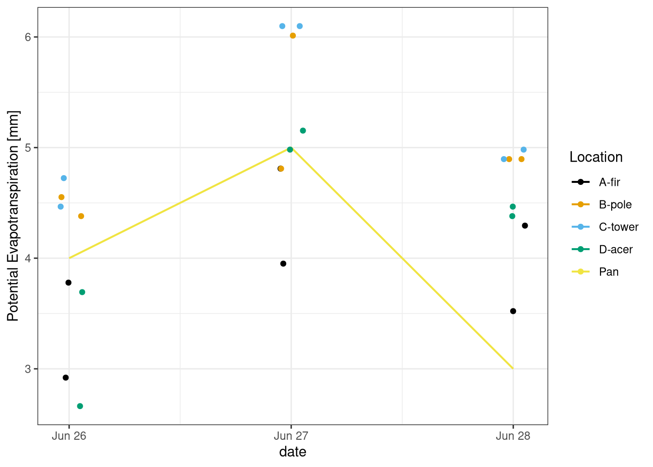
The potential ET (PET) has been measured using 8 Piché evaporimeters in 4 different locations around the botanical garden. Moreover a evaporation pan has aslo been used to measure the PET.

The piché evaporimeters were put in different location, some in the shade, some under the sunlight. Therefore a variation in the measured PET is expected (Figure 9.2), but overall the measures are comparable and is cleat that the ET on the 27th of June was higher.
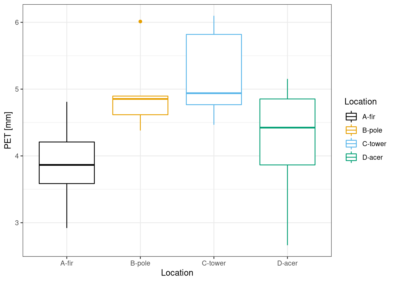
The piché evaporimeters between each other (Figure 9.3), it possible to see a reasonable pattern, for example the PET in the tower (exposed to the sun) is much higher than in the canopy of the fir. Finally the two evaporimeters in the same location report similar values for all location, but the fir. This is a confirmation that the field measurements are correct. The different measures may be related to problem in the piché evaporimeters sealing.

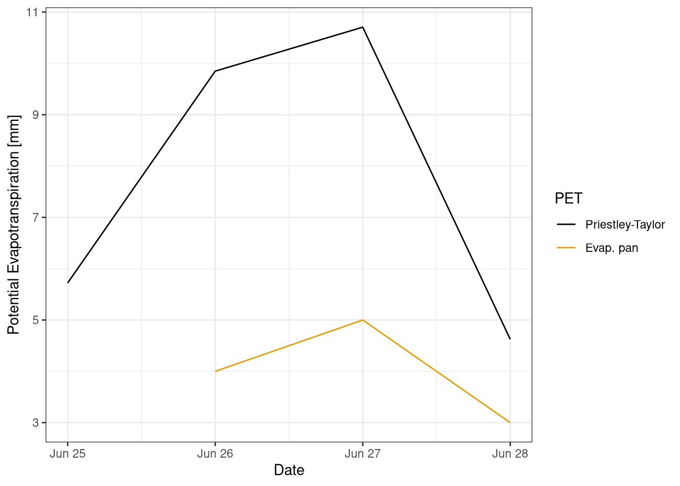
Finally the PET of the pan is compared with the PET estimated with the Priestley-Taylor equation (Figure 9.4). However, the values are very different with the PET from Priestley-Taylor being more than the double of the PET from the Pan. All the deta processing steps have been double checked but no explanation has been found for this difference.

pich_d <- 3 #cm
pich_inn_d <- 0.9 # cm
# calc area exposed to air:
# 2 times the area of the pare dish (two sides) - the area of glass
pich_dish_area <- 2 * (pi / 4 * pich_d ^ 2) - (pi / 4 * pich_inn_d ^ 2) # cm^2
# area inside the tube
pich_int_area <- (pi/4 * pich_inn_d ^2 ) # cm^2

et <- et %>% 
  group_by(loc_id) %>% 
  mutate(
    # here the scale is the opposite, the lower the number the more the water
    diff_pich = pich_height_cm - lag(pich_height_cm),
    # need to convert to mm of ET
    et_pich = diff_pich * pich_dish_area * pich_int_area / 10
  )

spot_cols <- hue_pal()(4)
names(spot_cols) <- unique(et$spot)
et %>% 
  drop_na() %>% #removing first empty day
ggplot(aes(date)) +
  geom_line(aes(y=et_pan, col="Pan"), size=.7) +
  geom_jitter(aes(y = et_pich, col=spot), width = .06, height = 0) +
  scale_color_manual(values=c(spot_cols, "Pan" = "black" )) +
  labs(y="Potential Evapotranspiration [mm]", colour="Location") +
  scale_color_colorblind()

Figure 9.2: Comparison of Potential Evapotranspiration between the evaporatin pan and 8 Piché evaporimeters in 4 different locations (fir, pole, tower, acer). Data from field measurement 26-28 June 2021.

et %>% 
  drop_na() %>% 
ggplot(aes(spot, et_pich, col=spot)) +
  geom_boxplot() +
  scale_color_colorblind() +
  labs(x='Location', y = "PET [mm]", col="Location")

Figure 9.3: PET at the different location. Data from field measurements 26-28 June 2021.

et %>% 
  left_join(meteo_d, by = c("date"= "Date")) %>% 
  gather("type", "et", PET, et_pan, factor_key = T) %>% 
  ggplot(aes(date, et, col=type)) +
  geom_line() +
  labs(y= "Potential Evapotranspiration [mm]", x="Date", col="PET") +
  scale_color_colorblind(labels = c("Priestley-Taylor", "Evap. pan"))

Figure 9.4: Comparison of the PET between the field measure with the evaporation pan and the estimation using the Priestley-Taylor equation. Data from field measurements and botanical garden 25-28 June 2021.