13 Regression Prediction
Let’s do one more example of an interaction using the ACS data:
load("Data/ACSCountyData.Rdata")How does the effect of the percent who commute by car on commute time change as population density increases?
What do we mean by this question. First, we think there is some sort of unconditional relationship between the percent of people who commute by transit and commuting time. Given that, in the US at least, transit commuting is a real second-class option, my expectation is that the more people who commute by transit in a location the longer average commute times will be.
We can confirm that using a bivariate regression:
library(stargazer)
#>
#> Please cite as:
#>  Hlavac, Marek (2018). stargazer: Well-Formatted Regression and Summary Statistics Tables.
#>  R package version 5.2.2. https://CRAN.R-project.org/package=stargazer
m <- lm(average.commute.time ~ percent.transit.commute, data=acs)
stargazer(m, type="text")
#>
#> ===================================================
#>                             Dependent variable:
#>                         ---------------------------
#>                            average.commute.time
#> ---------------------------------------------------
#> percent.transit.commute          0.353***
#>                                   (0.032)
#>
#> Constant                         23.225***
#>                                   (0.105)
#>
#> ---------------------------------------------------
#> Observations                       3,140
#> R2                                 0.037
#> Adjusted R2                        0.037
#> Residual Std. Error          5.630 (df = 3138)
#> F Statistic              121.671*** (df = 1; 3138)
#> ===================================================
#> Note:                   *p<0.1; **p<0.05; ***p<0.01
Indeed, for every additional percent of people commuting by transit average commute times increase by .353.
An objection to that regression might be that rural places have both low transit commuting and low commute times (if people work on their farms, for example). So we may want to take into account the indpendent effect of population density on both the percent who commute by transit and average commute times:
m2 <- lm(average.commute.time ~ percent.transit.commute + population.density, data=acs)
stargazer(m,m2, type="text")
#>
#> ==========================================================================
#>                                        Dependent variable:
#>                         --------------------------------------------------
#>                                        average.commute.time
#>                                    (1)                      (2)
#> --------------------------------------------------------------------------
#> percent.transit.commute         0.353***                  0.391***
#>                                  (0.032)                  (0.056)
#>
#> population.density                                        -0.0001
#>                                                           (0.0001)
#>
#> Constant                        23.225***                23.209***
#>                                  (0.105)                  (0.107)
#>
#> --------------------------------------------------------------------------
#> Observations                      3,140                    3,140
#> R2                                0.037                    0.038
#> Adjusted R2                       0.037                    0.037
#> Residual Std. Error         5.630 (df = 3138)        5.631 (df = 3137)
#> F Statistic             121.671*** (df = 1; 3138) 61.166*** (df = 2; 3137)
#> ==========================================================================
#> Note:                                          *p<0.1; **p<0.05; ***p<0.01
Actually this relationship gets stronger once we take into account the independent effect of population density.
But that’s not the question we asked, we want to know if the effect of the percent transit commuters changes as population density increases. To do that we have to multiply the two variables:
m3 <- lm(average.commute.time ~ percent.transit.commute*population.density, data=acs)

stargazer(m,m2,m3, type="text")
#>
#> ======================================================================================================================
#>                                                                        Dependent variable:
#>                                            ---------------------------------------------------------------------------
#>                                                                       average.commute.time
#>                                                       (1)                      (2)                      (3)
#> ----------------------------------------------------------------------------------------------------------------------
#> percent.transit.commute                            0.353***                  0.391***                 0.272***
#>                                                     (0.032)                  (0.056)                  (0.061)
#>
#> population.density                                                           -0.0001                  0.001***
#>                                                                              (0.0001)                 (0.0002)
#>
#> percent.transit.commute:population.density                                                          -0.00002***
#>                                                                                                      (0.00000)
#>
#> Constant                                           23.225***                23.209***                23.110***
#>                                                     (0.105)                  (0.107)                  (0.109)
#>
#> ----------------------------------------------------------------------------------------------------------------------
#> Observations                                         3,140                    3,140                    3,140
#> R2                                                   0.037                    0.038                    0.045
#> Adjusted R2                                          0.037                    0.037                    0.044
#> Residual Std. Error                            5.630 (df = 3138)        5.631 (df = 3137)        5.610 (df = 3136)
#> F Statistic                                121.671*** (df = 1; 3138) 61.166*** (df = 2; 3137) 49.045*** (df = 3; 3136)
#> ======================================================================================================================
#> Note:                                                                                      *p<0.1; **p<0.05; ***p<0.01
Ok we have lots of start here, so let’s break down what it is that we are seeing here.
The intercept here is 23.110. I have said many times that the intercept is the average value of the outcome when all variables in the regression are equal to 0, so this is the average commute time in a place with 0 transit commuters and 0 population density. So, as often is this case, this is a nonsense number.
To get the effect of the percent commuting by transit we can deploy a derivative:
\[ \hat{commute} = \alpha + \beta_1 Transit + \beta_@ Dens + \beta_3 Transity*Dens\\ \frac{\partial\hat{commute} }{\partial Transit} = \beta_1 + \beta_3*Dens\\ \]
As we wanted, the effect of the percent who commute by transit changes across levels of population density. If this equation describes the effect of % transit, under what conditions is the effect \(\beta_1\)? This is only the case when population density is equal to 0. So in a county with zero people the effect of an additional transit commuter is to increase average commute times by .272. Is this an important number? No! You have to know to ignore this number.
To determine what the effect of percent transit commute is, we have to evaluate at many values of of population density. Again, we have to be smart here. Try to think: what values does density take on?
summary(acs$population.density)
#>     Min.  1st Qu.   Median     Mean  3rd Qu.     Max.
#>     0.04    16.69    44.72   270.68   116.71 72052.96
OK! Let’s just do the math:
population.density <- seq(0,73000,1)
marginal.effect <- coef(m3)["percent.transit.commute"] + population.density*coef(m3)["percent.transit.commute:population.density"]

plot(population.density, marginal.effect, type="l", xlab="Population Density", ylab="Effect of % Transit Commute on Commute Time")
abline(h=0, lty=2)
rug(acs$population.density)
We see that this line is negative. This is saying that the effect of percent commuting by transit decreases as population density increases. In other words, when a place gets more dense having more people commute by transit moves from a net time suck on commute times to a net positive.
I have added the rug plot here to show where counties population densities actually are, and that rug plot somewhat tempers this finding. The truth is that the majority of counties have very small population densities and so this negative relationship is not true for many places.
This graph is not particularly helpful without some sense of the error. Can we conclude with any certainty that the effect of the percent commuting by transit on commute times is truly negative at any point?
What is the variance of this marginal effect? In other words what is:
\[ V(\beta_1 + \beta_3*Dens)=? \]
Is it just:
\[ V(\beta_1 + \beta_3*Dens) \neq V(\beta_1) + V(\beta_3*Dens) \]
No! When we are adding variance we critically need to know if there is any covariance between the two things. That is because:
\[ V(X+Y) = V(X) + V(Y) + 2*COV(X,Y) \]
So we could ignore the covariance if there was 0 covariance between these two features. Do the coefficients co-vary? Let’s simulate via bootstrap to see if beta 1 and beta 3 covary:
small <- acs[c("percent.transit.commute","population.density","average.commute.time")]
b1 <- rep(NA, 1000)
b3 <- rep(NA, 1000)
for(i in 1:1000){
  bs.data <- small[sample(1:nrow(small), nrow(small),replace=T),]
  m.bs <- lm(average.commute.time ~ percent.transit.commute*population.density, data=bs.data)
  b1[i] <- coef(m.bs)["percent.transit.commute"]
  b3[i] <- coef(m.bs)["percent.transit.commute:population.density"]
}
cor(b1,b3)
#> [1] 0.1535127
Yes! There is a non-zero correlation between these two things.
As such the variance of the marginal effect is:
\[ V(\beta_1 + \beta_3*Dens) = V(\beta_1) + V(\beta_3*Dens) + 2*Cov(\beta_1, \beta_3*Dens)\\ = V(\beta_1) + Dens^2*V(\beta_3) + 2*Dens*Cov(\beta_1, \beta_3)\\ \]
Notice how population density is a variable in this equation. The standard error of the marginal effect changes across levels of density. We will see this visually in a second.
How can we get these variances and co-variances?
vcov(m3)
#>                                              (Intercept)
#> (Intercept)                                 1.177826e-02
#> percent.transit.commute                    -1.378290e-03
#> population.density                         -2.825708e-06
#> percent.transit.commute:population.density  7.390022e-08
#>                                            percent.transit.commute
#> (Intercept)                                          -1.378290e-03
#> percent.transit.commute                               3.752489e-03
#> population.density                                   -1.011826e-05
#> percent.transit.commute:population.density            8.850673e-08
#>                                            population.density
#> (Intercept)                                     -2.825708e-06
#> percent.transit.commute                         -1.011826e-05
#> population.density                               6.223717e-08
#> percent.transit.commute:population.density      -8.328641e-10
#>                                            percent.transit.commute:population.density
#> (Intercept)                                                              7.390022e-08
#> percent.transit.commute                                                  8.850673e-08
#> population.density                                                      -8.328641e-10
#> percent.transit.commute:population.density                               1.316543e-11
The “variance-covariance” matrix is generated by the regression and tells us the variances (the diagonals) and the covariances (the off diaganoals) of all of the coefficients including the intercept.
So to get the standard error of the marginal effect at all the levels we calculated above:
var.margin <- vcov(m3)["percent.transit.commute","percent.transit.commute"] +
              population.density^2*vcov(m3)["percent.transit.commute:population.density","percent.transit.commute:population.density"] +
              population.density*2*vcov(m3)["percent.transit.commute:population.density","percent.transit.commute"]
This is variance, so to get the standard errors we take the square root:
se.margin <- sqrt(var.margin)Each entry here is the standard deviation of the sampling distribution at that point. If each of those sampling distributions is normally distributed, then the 95% confidence interval will run 1.96 standard errors above and below our estimate:
upper.bounds <- marginal.effect +se.margin*1.96
lower.bounds <- marginal.effect - se.margin*1.96
Now for this graph we
population.density <- seq(0,73000,1)
marginal.effect <- coef(m3)["percent.transit.commute"] + population.density*coef(m3)["percent.transit.commute:population.density"]

plot(population.density, marginal.effect, type="l", xlab="Population Density", ylab="Effect of % Transit Commute on Commute Time")
abline(h=0, lty=2)
points(population.density, upper.bounds, type="l", lty=2)
points(population.density, lower.bounds, type="l", lty=2)
rug(acs$population.density)
This should be the same as what we get in the margins package:
library(margins)
#> Warning: package 'margins' was built under R version 4.1.3
cplot(m3, x="population.density",dx="percent.transit.commute", what="effect")
abline(h=0)
13.1 Predicting with regression
The same ability to draw a line on a graph of data also allows us to use regression to make predictions about out of sample information.
library(lubridate)
#> Warning: package 'lubridate' was built under R version
#> 4.1.3
#>
#> Attaching package: 'lubridate'
#> The following objects are masked from 'package:base':
#>
#>     date, intersect, setdiff, union
mwr <- read.csv("Data/MarathonWR.csv")

#Some cleaning because I copied data from wikipedia
names(mwr) <- c("time","date")
mwr <- mwr[-5,]
mwr$seconds <- seconds(hms(mwr$time))
mwr$date <- dmy(mwr$date)
mwr$date[1:30] <- mwr$date[1:30]-years(100)
mwr$year <- year(mwr$date)
mwr$seconds <- as.numeric(mwr$seconds)
mwr$year <- as.numeric(mwr$year)

#How many seconds is 2 hours?
2*3600
#> [1] 7200

#Plotting this relationship:
library(ggplot2)
#> Warning: package 'ggplot2' was built under R version 4.1.3
p <- ggplot(mwr, aes(x=year, y=seconds)) + geom_point() +
  labs(x="Date", y = "Time") +
  geom_smooth(method = lm, formula = y ~ poly(x, 1), se = FALSE)
p
m <- lm(seconds ~ year, data=mwr)
summary(m)
#>
#> Call:
#> lm(formula = seconds ~ year, data = mwr)
#>
#> Residuals:
#>    Min     1Q Median     3Q    Max
#> -410.6 -188.4 -100.2  166.1  944.4
#>
#> Coefficients:
#>              Estimate Std. Error t value Pr(>|t|)
#> (Intercept) 54898.384   2406.743   22.81   <2e-16 ***
#> year          -23.755      1.227  -19.36   <2e-16 ***
#> ---
#> Signif. codes:
#> 0 '***' 0.001 '**' 0.01 '*' 0.05 '.' 0.1 ' ' 1
#>
#> Residual standard error: 291.5 on 48 degrees of freedom
#> Multiple R-squared:  0.8865, Adjusted R-squared:  0.8842
#> F-statistic:   375 on 1 and 48 DF,  p-value: < 2.2e-16
Now, ignoring that this is not a very good fit, we can use the output of this regression to predict future years marathon times.
future.years <- seq(2023,2050,1)

prediction <- coef(m)["(Intercept)"] + coef(m)["year"]*future.years

cbind(future.years, prediction/3600)
#>       future.years
#>  [1,]         2023 1.900505
#>  [2,]         2024 1.893906
#>  [3,]         2025 1.887308
#>  [4,]         2026 1.880709
#>  [5,]         2027 1.874110
#>  [6,]         2028 1.867512
#>  [7,]         2029 1.860913
#>  [8,]         2030 1.854314
#>  [9,]         2031 1.847716
#> [10,]         2032 1.841117
#> [11,]         2033 1.834518
#> [12,]         2034 1.827920
#> [13,]         2035 1.821321
#> [14,]         2036 1.814722
#> [15,]         2037 1.808124
#> [16,]         2038 1.801525
#> [17,]         2039 1.794927
#> [18,]         2040 1.788328
#> [19,]         2041 1.781729
#> [20,]         2042 1.775131
#> [21,]         2043 1.768532
#> [22,]         2044 1.761933
#> [23,]         2045 1.755335
#> [24,]         2046 1.748736
#> [25,]         2047 1.742137
#> [26,]         2048 1.735539
#> [27,]         2049 1.728940
#> [28,]         2050 1.722342
What is the confidence interval around each of these predictions?
We can use the same insite above:
\[ V(\alpha + \beta*years)=V(\alpha) + years^2 *V(\beta) + 2*years*Cov(\alpha,\beta) \]
var <- vcov(m)["(Intercept)","(Intercept)"] + future.years^2 * vcov(m)["year","year"] + 2*future.years * vcov(m)["year","(Intercept)"]
se.pred <- sqrt(var)
upper <- (prediction + se.pred*1.96)/3600
lower <- (prediction - se.pred*1.96)/3600


plot(future.years, prediction/3600, type="l", ylim=c())
points(future.years, lower, type="l", lty=2)
points(future.years, upper, type="l", lty=2)
Thankfully we can simplify this procedure greatly using the predict() command.
In it’s basic form predict will spit out the value of the line for all of your data points
mwr$prediction <-  predict(m)
head(mwr)
#>      time       date seconds year prediction
#> 1 2:55:18 1908-07-24   10518 1908   9573.654
#> 2 2:52:45 1909-01-01   10365 1909   9549.899
#> 3 2:46:53 1909-02-12   10013 1909   9549.899
#> 4 2:46:05 1909-05-08    9965 1909   9549.899
#> 6 2:40:34 1909-08-31    9634 1909   9549.899
#> 7 2:38:16 1913-05-12    9496 1913   9454.878
But helpfully we can also feed new data into the predict function with new values for the x variable
prediction2 <- predict(m, newdata=data.frame(year=future.years))
cbind(prediction, prediction2)
#>    prediction prediction2
#> 1    6841.817    6841.817
#> 2    6818.062    6818.062
#> 3    6794.307    6794.307
#> 4    6770.552    6770.552
#> 5    6746.797    6746.797
#> 6    6723.042    6723.042
#> 7    6699.287    6699.287
#> 8    6675.532    6675.532
#> 9    6651.776    6651.776
#> 10   6628.021    6628.021
#> 11   6604.266    6604.266
#> 12   6580.511    6580.511
#> 13   6556.756    6556.756
#> 14   6533.001    6533.001
#> 15   6509.246    6509.246
#> 16   6485.491    6485.491
#> 17   6461.736    6461.736
#> 18   6437.981    6437.981
#> 19   6414.225    6414.225
#> 20   6390.470    6390.470
#> 21   6366.715    6366.715
#> 22   6342.960    6342.960
#> 23   6319.205    6319.205
#> 24   6295.450    6295.450
#> 25   6271.695    6271.695
#> 26   6247.940    6247.940
#> 27   6224.185    6224.185
#> 28   6200.430    6200.430
What’s more, the predict function will also determine the confidence interval for you:
prediction2 <- predict(m, newdata=data.frame(year=future.years), interval="confidence")All of this is particularly helpful when calculating the predicted values are particularly difficult.
Above we can see that the linear regression is not a very good fit for these data. Instead, i’m going to propose that a 3rd order polynomial fit is what is best to fit to these data. That would look like this:
#Plotting this relationship:
library(ggplot2)
p <- ggplot(mwr, aes(x=year, y=seconds)) + geom_point() +
  labs(x="Date", y = "Time") +
  geom_smooth(method = lm, formula = y ~ poly(x, 3), se = FALSE)
p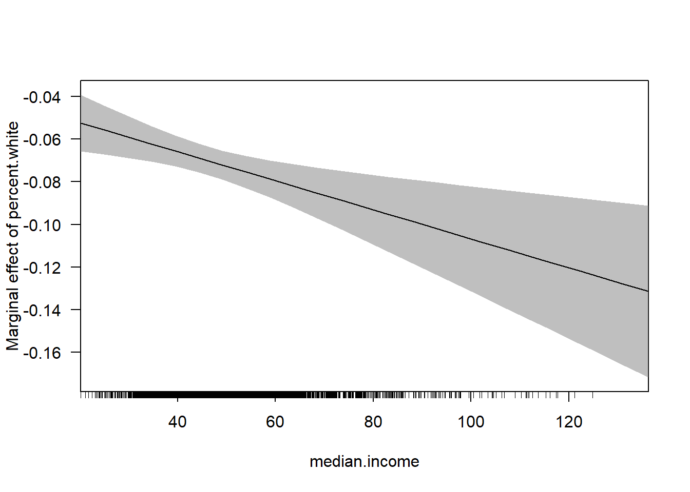
m2 <- lm(seconds ~ poly(year, 3), data=mwr)
summary(m2)
#>
#> Call:
#> lm(formula = seconds ~ poly(year, 3), data = mwr)
#>
#> Residuals:
#>     Min      1Q  Median      3Q     Max
#> -357.07  -41.24   18.96   48.94  526.26
#>
#> Coefficients:
#>                Estimate Std. Error t value Pr(>|t|)
#> (Intercept)     8298.48      22.67 366.133  < 2e-16 ***
#> poly(year, 3)1 -5644.47     160.27 -35.219  < 2e-16 ***
#> poly(year, 3)2  1678.50     160.27  10.473 9.16e-14 ***
#> poly(year, 3)3  -281.26     160.27  -1.755   0.0859 .
#> ---
#> Signif. codes:
#> 0 '***' 0.001 '**' 0.01 '*' 0.05 '.' 0.1 ' ' 1
#>
#> Residual standard error: 160.3 on 46 degrees of freedom
#> Multiple R-squared:  0.9671, Adjusted R-squared:  0.965
#> F-statistic: 451.1 on 3 and 46 DF,  p-value: < 2.2e-16
It’s not too bad to use the math to predict the fitted values for all of the future years, but calculating the standard error for the confidence band at each of those fitted values would be extremely difficult.
Thankfully, we can just pipe in the model to the predict function and generate predictions and a confidence interval around those predictions:
prediction.poly <- predict(m2, newdata=data.frame(year=future.years), interval="confidence")
plot(future.years, prediction.poly[,1], type="l", ylim=c(6000,8000))
points(future.years, prediction.poly[,2], type="l")
points(future.years, prediction.poly[,3], type="l")
abline(h=7200, lty=3)
Displayed with all the data:
prediction.poly <- predict(m2, newdata=data.frame(year=future.years), interval="confidence")
plot(future.years, prediction.poly[,1], type="l", ylim=c(6000,11000), xlim=c(1900,2050))
points(future.years, prediction.poly[,2], type="l")
points(future.years, prediction.poly[,3], type="l")
points(mwr$year, mwr$seconds, pch=16)
abline(h=7200, lty=3)
13.2 Out of Sample Prediction
Let’s go through another example of making out of sample predictions.
In order to conduct a pre-election survey a necessary step is to predict who is likely to vote and who is not. This is critical because a pre-election poll is not meant to predict the opinions of all Americans, but rather the opinions of voters specifically. Making a judgement on who that is a critical step.
We are going to look at building a likely voter model using CCES data. One of the nice things about the CCES is that, post election, they use the voter file to determine who actually voted out of the people that they surveyed. This is great information because people lie like crazy when we ask them if they voted or not.
load("Data/CCES.Rdata")
cces <- cces.class
head(cces)
#> # A tibble: 6 x 9
#>    year vv.turnout educ    white female agegrp vote.~1 pid3
#>   <int>      <int> <chr>   <chr>  <dbl> <fct>  <chr>   <fct>
#> 1  2016          1 HS or ~ white      1 40-49  Maybe   3
#> 2  2016          1 HS or ~ white      1 18-29  Yes     3
#> 3  2016          0 HS or ~ nonw~      1 50-64  Yes     1
#> 4  2016          1 HS or ~ nonw~      1 18-29  Yes     3
#> 5  2016          1 college white      1 30-39  Yes     1
#> 6  2016          0 HS or ~ nonw~      1 50-64  Maybe   1
#> # ... with 1 more variable: prim.turnout <dbl>, and
#> #   abbreviated variable name 1: vote.intent
table(cces$year)
#>
#>  2016  2018  2020
#> 64600 60000 61000
The models we want to build here are to predict vv.turnout, whether someone voted (1) or not (0). So for example, taking the 2016 voters, we can determine how an individual’s vote intention predicts whether they will vote, or not.
table(cces$vote.intent)
#>
#> Already voted         Maybe            No           Yes
#>         16563         23491         15139        130199
cces$vote.intent <- factor(cces$vote.intent)
cces$vote.intent <- relevel(cces$vote.intent, ref="No")

cces.16 <- cces[cces$year==2016,]
m <- lm(vv.turnout ~ vote.intent, data=cces.16)
summary(m)
#>
#> Call:
#> lm(formula = vv.turnout ~ vote.intent, data = cces.16)
#>
#> Residuals:
#>     Min      1Q  Median      3Q     Max
#> -0.6969 -0.6499  0.3502  0.3502  0.9261
#>
#> Coefficients:
#>                          Estimate Std. Error t value
#> (Intercept)              0.073882   0.006337   11.66
#> vote.intentAlready voted 0.623028   0.013332   46.73
#> vote.intentMaybe         0.174263   0.008153   21.37
#> vote.intentYes           0.575972   0.006660   86.48
#>                          Pr(>|t|)
#> (Intercept)                <2e-16 ***
#> vote.intentAlready voted   <2e-16 ***
#> vote.intentMaybe           <2e-16 ***
#> vote.intentYes             <2e-16 ***
#> ---
#> Signif. codes:
#> 0 '***' 0.001 '**' 0.01 '*' 0.05 '.' 0.1 ' ' 1
#>
#> Residual standard error: 0.4575 on 64484 degrees of freedom
#>   (112 observations deleted due to missingness)
#> Multiple R-squared:  0.1528, Adjusted R-squared:  0.1528
#> F-statistic:  3877 on 3 and 64484 DF,  p-value: < 2.2e-16
Because the intercept is the probability of voting when all other variables are 0, this is the probability of voting for someone who said they would not vote in the upcoming election (about 7.3%). Each of these coefficients indicates the change of probability of moving from being an expressed non-voter to each of those categories. We can do the math ourselves or use predict:
predict(m, newdata= data.frame(vote.intent=c("No", "Maybe", "Yes", "Already voted")))
#>          1          2          3          4
#> 0.07388217 0.24814489 0.64985443 0.69690993
So for the 2016 data only 70% of those who said they already voted actually voted. The lies!
Now pretend that it’s fall of 2020 and we have collected the data but the election hasn’t happened yet. How can we use the other data to predict, for the 2020 respondents, whether they are going to vote or not. Now we actually have this information and can verify how we do with our predictions, but that’s not something that would actually be available to us at the time.
Let’s use the 2016 and 2018 data to build a couple of models that predict whether someone voted or not. I’m going to use 4 models from simple to complex:
cces.training <- cces[cces$year %in% c(2016,2018),]
cces.test <- cces[cces$year==2020,]
m1 <- lm(vv.turnout ~ vote.intent, data=cces.training)
m2 <- lm(vv.turnout ~  vote.intent +prim.turnout + educ:white, data=cces.training)
m3 <- lm(vv.turnout ~ female + vote.intent +prim.turnout + educ:white:agegrp + pid3, data=cces.training)
These are 3 models with increasingly complicated equations. We haven’t seen regressions with this many variables but, rest assured, everything we’ve talked about so far applies. These are (mostly) just a series of indicator variables and interactions.
The important thing here is that because the 2020 data has the exact same variables in it, we can use the coefficients in these models to form predictions in the 2020 data.
Consider the first model:
summary(m1)
#>
#> Call:
#> lm(formula = vv.turnout ~ vote.intent, data = cces.training)
#>
#> Residuals:
#>     Min      1Q  Median      3Q     Max
#> -0.7710 -0.6675  0.3325  0.3325  0.9336
#>
#> Coefficients:
#>                          Estimate Std. Error t value
#> (Intercept)              0.066432   0.004318   15.39
#> vote.intentAlready voted 0.704534   0.007914   89.02
#> vote.intentMaybe         0.175119   0.005477   31.97
#> vote.intentYes           0.601085   0.004565  131.67
#>                          Pr(>|t|)
#> (Intercept)                <2e-16 ***
#> vote.intentAlready voted   <2e-16 ***
#> vote.intentMaybe           <2e-16 ***
#> vote.intentYes             <2e-16 ***
#> ---
#> Signif. codes:
#> 0 '***' 0.001 '**' 0.01 '*' 0.05 '.' 0.1 ' ' 1
#>
#> Residual standard error: 0.4482 on 124444 degrees of freedom
#>   (152 observations deleted due to missingness)
#> Multiple R-squared:  0.1851, Adjusted R-squared:  0.1851
#> F-statistic:  9423 on 3 and 124444 DF,  p-value: < 2.2e-16
predict(m1, newdata= data.frame(vote.intent=c("No", "Maybe", "Yes", "Already voted")))
#>          1          2          3          4
#> 0.06643162 0.24155081 0.66751633 0.77096562
The people in 2020 also have a variable named vote.intent with the same response labels. As such we can do:
cces.test$predict1 <- predict(m1, newdata=cces.test)
head(cces.test)
#> # A tibble: 6 x 10
#>    year vv.turnout educ    white female agegrp vote.~1 pid3
#>   <int>      <int> <chr>   <chr>  <dbl> <fct>  <fct>   <fct>
#> 1  2020          1 some c~ white      0 50-64  Alread~ 2
#> 2  2020          0 postgr~ white      1 65-74  No      1
#> 3  2020          0 college white      1 65-74  Yes     3
#> 4  2020          1 college white      1 50-64  Yes     1
#> 5  2020          0 college white      0 50-64  Yes     3
#> 6  2020          1 some c~ white      0 50-64  Yes     2
#> # ... with 2 more variables: prim.turnout <dbl>,
#> #   predict1 <dbl>, and abbreviated variable name
#> #   1: vote.intent
table(cces.test$predict1)
#>
#> 0.066431619966184 0.241550808184305 0.667516327713994
#>              4361              5797             38790
#> 0.770965622946551
#>             11996
The predict1 column takes on 4 possible values based on the individuals vote intention.
We can classify each person as a likely voter or not if there probability of voting is above or below 50%. From that we can determine how good of a job this model does in predicting 2020 voters. We can look to see the proportion of voters who are incorrectly classified. IE, how many are predicted to vote but don’t, and how many are predicted not to vote but do?
#Classification Error
mean((cces.test$predict1>.5 & cces.test$vv.turnout==0) | (cces.test$predict1<.5 & cces.test$vv.turnout==1),na.rm=T)
#> [1] 0.2363153
The two other models both have a substantially higher \(R^2\), meaning that the models fit the 2016/2018 data much better. The question is whether this better fitting data also reduces the classification error. Notice that even though these models have lots of complicated interactions and many variables the code to actually form predictions is really easy! Wee! Regression is fun!
cces.test$predict2 <- predict(m2, newdata=cces.test)
#> Warning in predict.lm(m2, newdata = cces.test): prediction
#> from a rank-deficient fit may be misleading
cces.test$predict3 <- predict(m3, newdata=cces.test)
#> Warning in predict.lm(m3, newdata = cces.test): prediction
#> from a rank-deficient fit may be misleading

#Classification Error Model 2
mean((cces.test$predict2>.5 & cces.test$vv.turnout==0) | (cces.test$predict2<.5 & cces.test$vv.turnout==1),na.rm=T)
#> [1] 0.2115221

#Classification Error Model 3
mean((cces.test$predict3>.5 & cces.test$vv.turnout==0) | (cces.test$predict3<.5 & cces.test$vv.turnout==1),na.rm=T)
#> [1] 0.1940142
Yes, in this case we do make a few fewer classification errors when we better fit the data. But let’s go crazy with this interacting everything we everything:
#Stupid model
m4 <- lm(vv.turnout ~ pid3:vote.intent:prim.turnout + female:educ:white:agegrp, data=cces.training)
cces.test$predict4<- predict(m4, newdata=cces.test)

#Classification Error Model 4
mean((cces.test$predict4>.5 & cces.test$vv.turnout==0) | (cces.test$predict4<.5 & cces.test$vv.turnout==1),na.rm=T)
#> [1] 0.2268804
It went back up!
Sum this up.
13.3 Summary
Where we started:
At some point in learning about statistics or data science you may have heard instructors talk about samples and the population. The purpose of this class is to think a lot between the relationships between these two things and to focus our minds on the idea that this interplay is actually what the whole enterprise is all about.
What defines statistics is making conclusions about populations from a sample of data. (We infer things about populations from samples, hence the title of the class.)
“Population” is a pretty vague term however, and it encompasses a really wide range of things.
Sometimes what we mean is very obvious: In politics we often take random samples of a few thousand people to help us to understand the opinions and attitudes of the entire United States. In this case it’s quite clear that the sample is the random sample of people while the population is the adult public of the United States.
But lots of other things in our day-to-day lives are “samples” from some population, we often just don’t consider them as such.
For example: we might be interested in learning about the revenue potential of a small business, and have a few months of their finances as data. The goal is to use this sample of data (which may or may not be perfectly representative!) to better understand what the true earning potential of that business is. In this case the “population” is simply the true earning potential of the business.
If you are sports inclined we can think of the performance of a baseball hitter over a certain stretch of time as a “Sample” from the population that is their true hitting potential.
If it’s helpful (it is for me sometimes) we can re-frame the “population” as the “data generating process”. In the baseball example there is an underlying truth (the hitter’s true skill) which generates data (if the player hits the ball or not) when they step up to the plate.
In statistics, we look to make probabilistic inferences from samples about unknowable truths about the world. We will never precisely know the earning potential of a business, or how many Americans support a presidential candidate, or what level of hitting skill a baseball player has. We can, however, form estimates from a sample of data and estimate our level of uncertainty about the degree to which our answer represents the truth.
Where do you go from here. There are, broadly, three extensions from this material that you can go to from here.
Pure statistics: there is a lot more in terms of probability, probability distributions, getting standard errors right etc. We have scratched the surface.
Causal inference: very exciting new field.
Prediction: Machine learning baby!