4.6 Simulation

We will consider two different simulations:

1. random walk model, and
2. Roll model of security price.

4.6.1 Random Walk

We first construct a random walk function that simulates random walk model. It takes the number of period (N), initial value (x0), drift (mu), and variance. The function use rnorm() to generate random normal variable, and then use cumsum() to get the random walk. Note that the whole function is based on vector operation, instead of looping over time.

RW <- function(N, x0, mu, variance) {
  z<-cumsum(rnorm(n=N, mean=0, 
                  sd=sqrt(variance)))
  t<-1:N
  x<-x0+t*mu+z
  return(x)
  }
# mu is the drift

P1<-RW(100,10,0,0.0004)
P2<-RW(100,10,0,0.0004)
plot(P1, main="Random Walk without Drift", 
     xlab="t",ylab="Price", ylim=c(9.7,10.3),
     typ='l', col="red")
par(new=T)  #to draw in the same plot
plot(P2, main="Random Walk without Drift", 
     xlab="t",ylab="Price", ylim=c(9.7,10.3),
     typ='l', col="blue")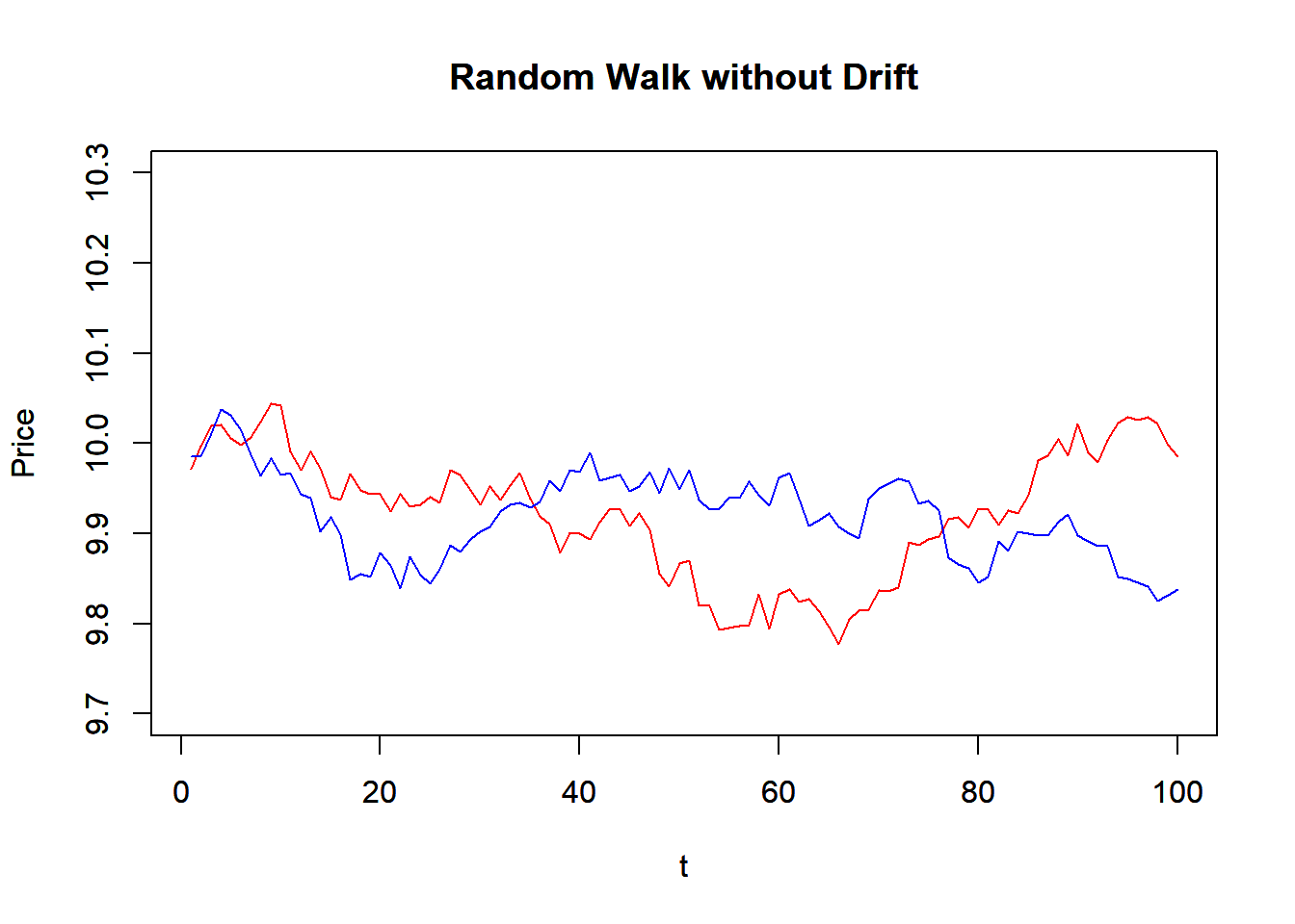

par(new=F)

4.6.2 Roll Model

To simulate the Roll model, we first simulate the price series and simulated trade prices. We calculate the first difference of the price and then we can estimate the first and the second orders of autocovariances. Then we can compare the true trading cost with the estimate one.

require(zoo)

trial <-1000  #Number of trial

cost <-c() #cost each trial
sd <-c()   #sd each trial

true.cost = 2
true.sd = 1

time = 1:trial

for (i in 1:trial) {
  
  #Simulated Price Series
  epsilon = rnorm(time,sd=true.sd)
  prices = cumsum(epsilon)
  m_t = zoo(prices)
  a_t = m_t + true.cost
  b_t = m_t - true.cost
  
  #simulated trade prices 
  q_t = sign(rnorm(time))
  p_t = m_t + (true.cost * q_t)
  
  #1st difference of prices
  delta_p <- p_t-lag(p_t)  
  #omit n.a. entry
  delta_p <- na.omit(delta_p) 

  gamma_0 <- var(delta_p)
  gamma_1 <- cov(delta_p[1:length(delta_p)-1], 
                 delta_p[2:length(delta_p)])
  sigma_2 <- gamma_0 + 2 * gamma_1
  
  if(gamma_1 > 0){
    print("Error: Positive Autocovariance!")
  } else {
    cost <- append(cost,sqrt(-1*gamma_1))
    sd <-append(sd,sigma_2)
  }
}

# Stimulated Cost Plot

plot(cost)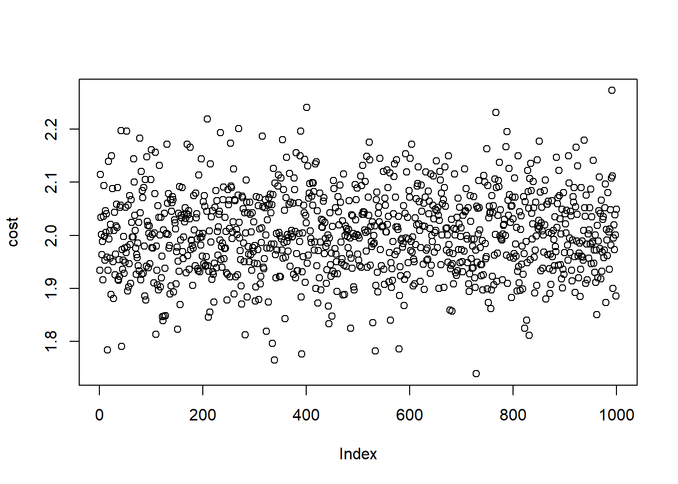

est.cost <- mean(cost)

plot(sd)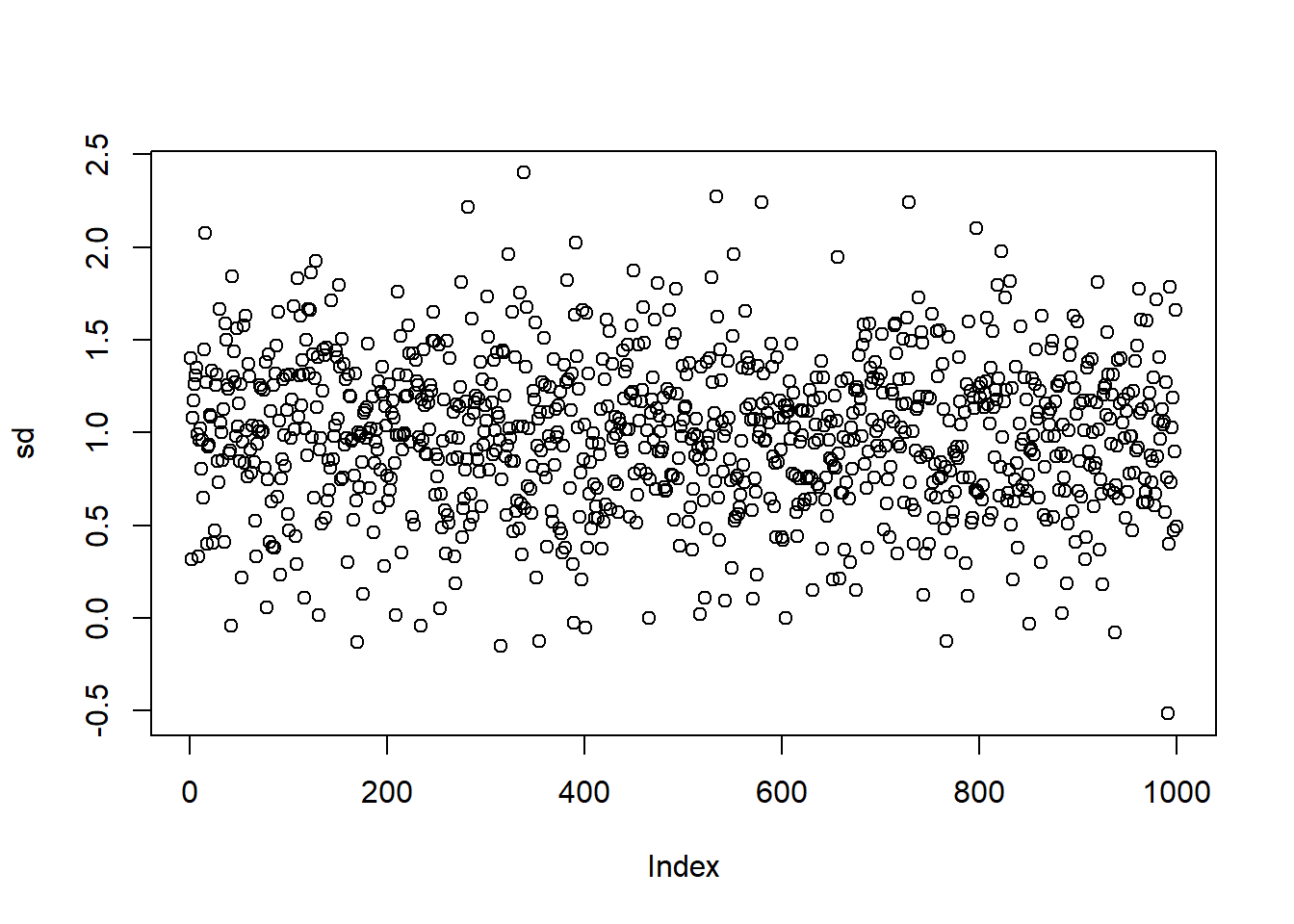

est.sd <- mean(sd)

# Final Result
cat("True cost and sd are", true.cost," and ", true.sd)

## True cost and sd are 2  and  1

cat("Estimated cost and sd are", est.cost," and ", est.sd)

## Estimated cost and sd are 2.003041  and  0.9919344