7.7 Evaluating Trading Rules
To simplify, we first evaluate several trading rules based on day trading:
- buy signal based on simple filter rule
- buy and sell signals based on simple filter rule
- buy signal based on RSI
- buy signal based on EMA and sell signal based on RSI
- buy signal based on RSI but trading size depends on price history
Finally, we consider the rule that does non-day trading. In this case, we need to keep track of both cash and stock holdings.
7.7.1 Simple filter Buy
Here we create trading signal based on simple filter rule. Recall that simple filter rule suggests buying when the price increases a lot compared to the yesterday price: \[\begin{align*} \text{Buy}&:\frac{P_t}{P_{t-1}}>1+\delta \\ \end{align*}\]where \(P_t\) is the closing price at time \(t\) and \(\delta>0\) is an arbitrary threshold
We illustrate using Microsoft with ticker MSFT.
We first download the data using getSymbols(“MSFT”).
library(quantmod)
getSymbols("MSFT")
## [1] "MSFT"We first will use closing price to perform calculation. We calculate the percentage price change by dividing the current close price by its own lag and then minus 1.
Now we generate buying signal based on filter rule:
price <- Cl(MSFT) # close price
r <- price/Lag(price) - 1 # % price change
delta <-0.005 #threshold
signal <-c(0) # first date has no signal

#Loop over all trading days (except the first)
for (i in 2: length(price)){
  if (r[i] > delta){
    signal[i]<- 1
  } else
    signal[i]<- 0
}
Note that signal is just a vector without time stamp. We use the function reclass to convert it into an xts object.
# Each data is not attached with time
head(signal, n=3)
## [1] 0 0 0# Assign time to action variable using reclass;
signal<-reclass(signal,price)
# Each point is now attached with time
tail(signal, n=3)## [,1]
## 2019-04-11 0
## 2019-04-12 1
## 2019-04-15 0We are now ready to chart the trading indicators:
# Charting with Trading rule
chartSeries(MSFT,
            type = 'line',
            subset="2009-08::2009-09-15",
            theme=chartTheme('white'))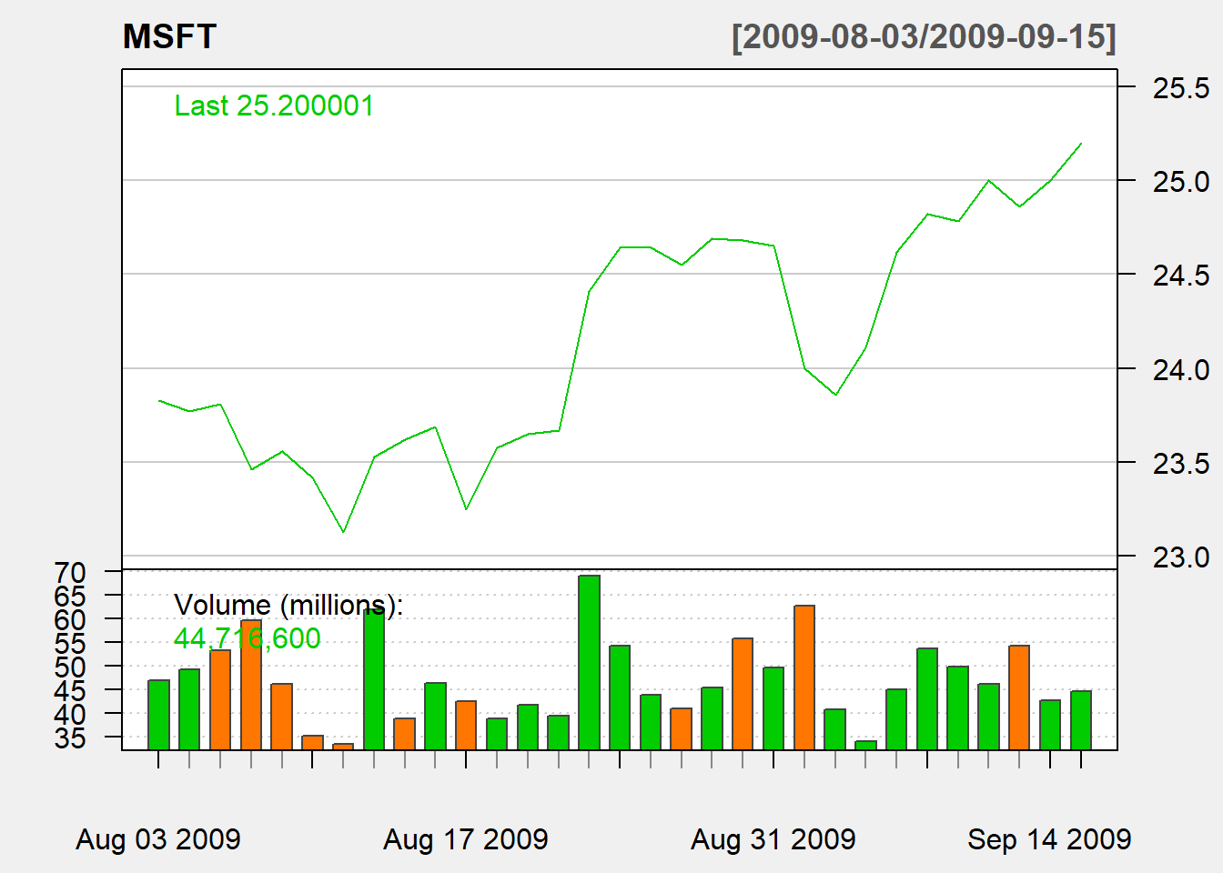
addTA(signal,type='S',col='red')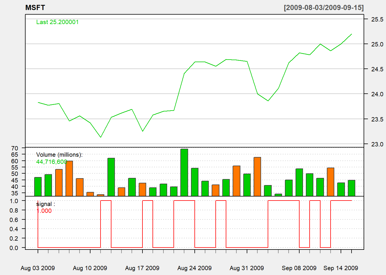
We consider trading based on yesterday indicator:
trade <- Lag(signal,1) # trade based on yesterday signalTo keep it simple, we evaluate using day trading:
- buy at open
- sell at close
- trading size: all in
Then daily profit rate is \(dailyReturn=\frac{Close - Open}{open}\)
ret<-dailyReturn(MSFT)*trade
names(ret)<-"filter"
Based on daily return, we can see the summary of performance using charts.PerformanceSummary() to evaluate the performance.
#Performance Summary
charts.PerformanceSummary(ret, main="Naive Buy Rule")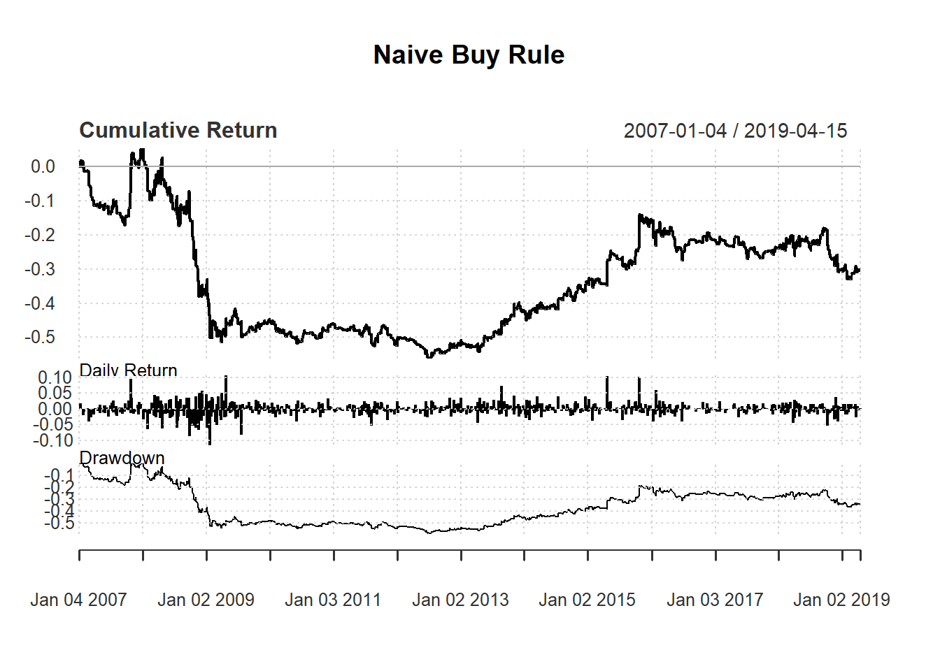
7.7.2 Simple fiter buy-sell
Here we create trading signal based on simple filter rule. Recall that simple filter rule suggests buying when the price increases a lot compared to the yesterday price and selling when price decreases a lot: \[\begin{align*} \text{Buy}&:\frac{P_t}{P_{t-1}}>1+\delta \\ \text{Sell}&:\frac{P_t}{P_{t-1}}<1-\delta \end{align*}\]where \(P_t\) is the closing price at time \(t\) and \(\delta>0\) is an arbitrary threshold
We first download the data:
library(quantmod)
getSymbols("MSFT")
## [1] "MSFT"price <- Cl(MSFT)
r <- price/Lag(price) - 1
delta<-0.005
signal <-c(NA) # first signal is NA
for (i in 2: length(Cl(MSFT))){
if (r[i] > delta){
signal[i]<- 1
} else if (r[i]< -delta){
signal[i]<- -1
} else
signal[i]<- 0
}
signal<-reclass(signal,Cl(MSFT))
trade1 <- Lag(signal)
ret1<-dailyReturn(MSFT)*trade1
names(ret1) <- 'Naive'
charts.PerformanceSummary(ret1)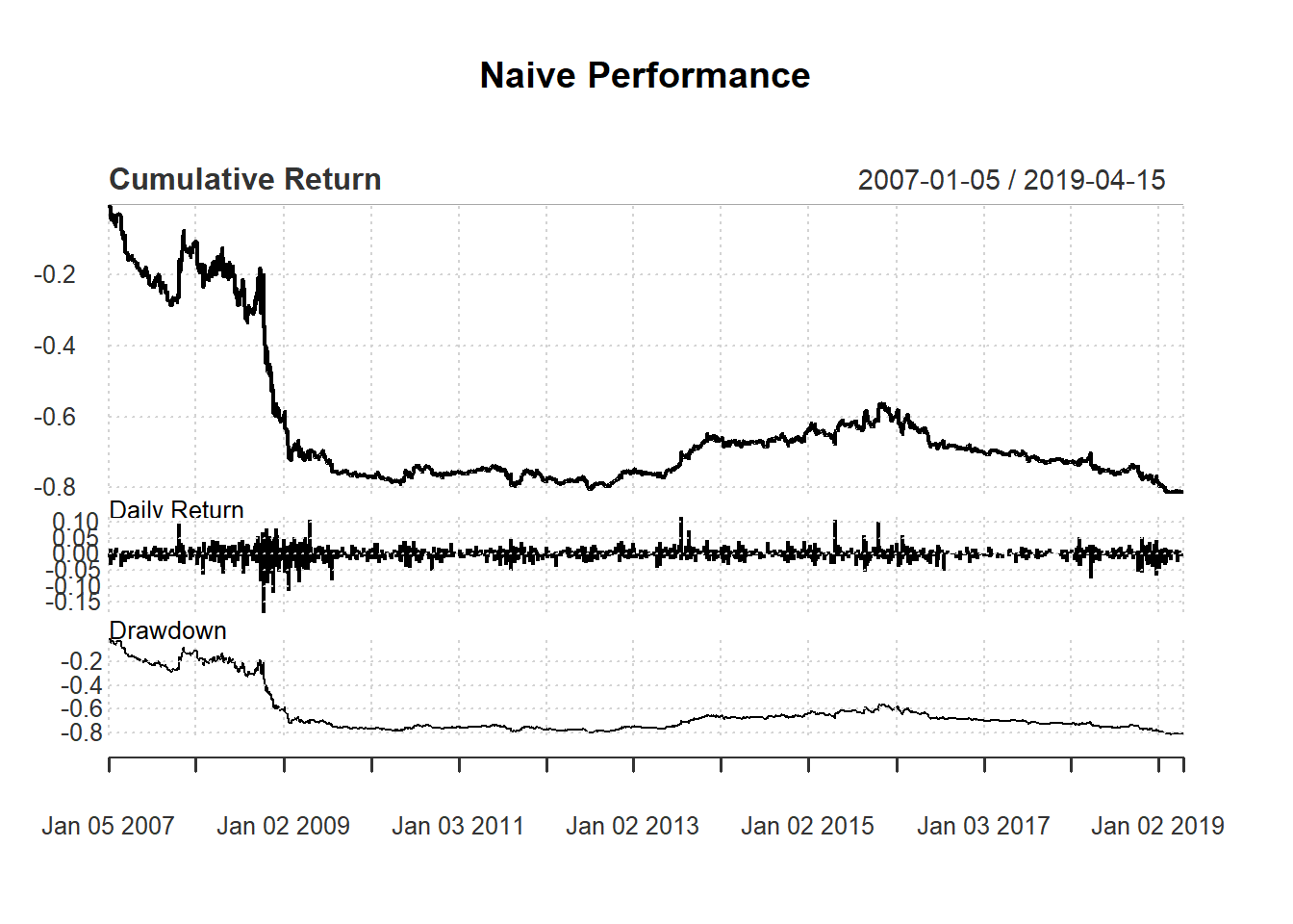
Exercise
Test the following strategy based on EMA: - Buy/Sell signal based on EMA rule. - Day trading based on yesterday signal: - buy at open and - sell at close on the same day
7.7.3 An example using RSI
Consider following day-trading strategy based on 14-day RSI:
- buy one unit if RSI <30 and
- otherwise no trade.
Evaluate this based on day trading and compare it with simple filter rule:
day <-14
price <- Cl(MSFT)
signal <- c()                    #initialize vector
rsi <- RSI(price, day)     #rsi is the lag of RSI
signal [1:day+1] <- 0            #0 because no signal until day+1

for (i in (day+1): length(price)){
  if (rsi[i] < 30){             #buy if rsi < 30
    signal[i] <- 1
  }else {                       #no trade all if rsi > 30
    signal[i] <- 0
  }
}
signal<-reclass(signal,Cl(MSFT))
trade2 <- Lag(signal)

#construct a new variable ret1
ret1 <- dailyReturn(MSFT)*trade1
names(ret1) <- 'Naive'
# construct a new variable ret2
ret2 <- dailyReturn(MSFT)*trade2
names(ret2) <- 'RSI'
Now compare strategies with the filter rule:
retall <- cbind(ret1, ret2)
charts.PerformanceSummary(retall,
                          main="Naive v.s. RSI")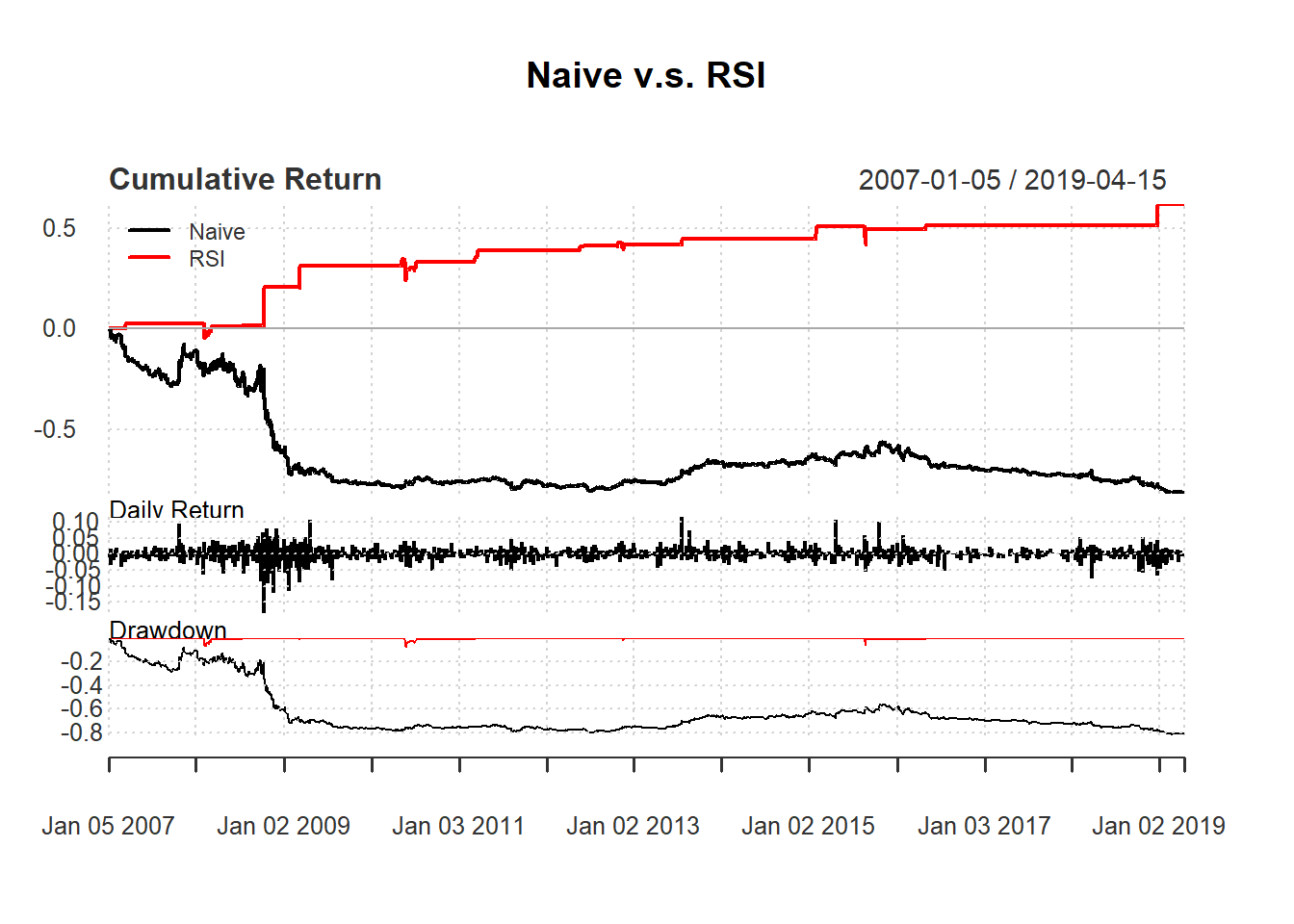
7.7.4 More efficient code
In the RSI code above, we have written that:
signal [1:day+1] <- 0

for (i in (day+1): length(price)){
  if (rsi[i] < 30){
    signal[i] <- 1
  }else {
    signal[i] <- 0
  }
}
A more efficient but less readable code is to avoid counting:
for (i in 1:length(price)){
  signal[i] <- 0
  if (isTRUE(rsi[i] < 30)){
    signal[i] <- 1
  }
}