8.3 Simple Filter Rule
8.3.1 Step 1: Initialization
We need to install standard packages and custom packages. After loading all the packages, we initialize are variables and then download data.
Then we need to get the data and define initial variables.Download using getSybmols()
options("getSymbols.warning4.0"=FALSE)
from ="2003-01-01"
to ="2012-12-31"
symbols = c("MSFT", "IBM")
getSymbols(symbols, from=from, to=to,
           adjust=TRUE)
Currency is USD for US stocks and the multiplier is always 1 for stocks.
currency("USD")
stock(symbols, currency="USD", multiplier=1)
We first define our strategy, portfolio and account name.
strategy.st <- "filter"
portfolio.st <- "filter"
account.st <- "filter"
Remove any old variables
rm.strat("filter")After naming strategy, portfolio and account, we initialize them:
initEq=100000
initDate="1990-01-01"

initPortf(name=portfolio.st,
          symbols=symbols,
          initDate=initDate,
          currency='USD')
initAcct(name=account.st,
         portfolios=portfolio.st,
         initDate=initDate,
         currency='USD',
         initEq=initEq)
initOrders(portfolio=portfolio.st,
           symbols=symbols,
           initDate=initDate)

strategy(strategy.st, store=TRUE)
8.3.2 Step 2: Define indicator
Indicator is just a function based on price. Since simple filter is not a standard technical indicator, we need to define it first.
filter <- function(price) {
  lagprice <- lag(price,1)
  temp<-price/lagprice - 1
  colnames(temp) <- "filter"
  return(temp)
}
We add the simple filter as an indicator. Here the name is the indicator function we have defined. We need to specify what data to be used by the indicator. Since we have defined that the simple filter rule takes price as input, we need to tell the problem we are using the closing price. Note that the label filter is the variable assigned to this indicator, which implies it must be unique.
add.indicator(
  strategy=strategy.st,
  name = "filter",
  arguments = list(price = quote(Cl(mktdata))),
  label= "filter")
To check if the indicator is defined correctly, use applyindicators to see if it works. The function try() is to allow the program continue to run even if there is an error.
test <-try(applyIndicators(strategy.st,
                           mktdata=OHLC(AAPL)))
head(test, n=4)
8.3.3 Step 3: Trading Signals
Trading signals is generated from the trading indicators. For example, simple trading rule dictates that there is a buy signal when the filter exceeds certain threshold.
In quantstrat, there are three ways one can use a signal. It is refer to as name:
- sigThreshold: more or less than a fixed value
- sigCrossover: when two signals cross over
- sigComparsion: compare two signals
The column refers to the data for calculation of signal. There are five possible relationship:
- gt = greater than
- gte = greater than or equal to
- lt = less than
- lte = less than or equal to
- eq = equal to
Buy Signal under simple trading rule with threshold \(\delta=0.05\)
# enter when filter > 1+\delta
add.signal(strategy.st,
           name="sigThreshold",
           arguments = list(threshold=0.05,
                            column="filter",
                            relationship="gt",
                            cross=TRUE),
           label="filter.buy")
Sell Signal under simple trading rule with threshold \(\delta=-0.05\)
# exit when filter < 1-delta
add.signal(strategy.st,
           name="sigThreshold",
           arguments = list(threshold=-0.05,
                            column="filter",
                            relationship="lt",
                            cross=TRUE),
           label="filter.sell")
8.3.4 Step 4. Trading Rules
While trading signals tell us buy or sell, but it does not specify the execution details.
Trading rules will specify the following seven elements:
- SigCol: Name of Signal
- SigVal: implement when there is signal (or reverse)
- Ordertype: market, stoplimit
- Orderside: long, short
- Pricemethod: market
- Replace: whether to replace other others
- Type: enter or exit the order
Buy rule specifies that when a buy signal appears, place a buy market order with quantity size.
add.rule(strategy.st,
         name='ruleSignal',
         arguments = list(sigcol="filter.buy",
                          sigval=TRUE,
                          orderqty=1000,
                          ordertype='market',
                          orderside='long',
                          pricemethod='market',
                          replace=FALSE),
         type='enter',
         path.dep=TRUE)
Sell rule specifies that when a sell signal appears, place a sell market order with quantity size.
add.rule(strategy.st,
         name='ruleSignal',
         arguments = list(sigcol="filter.sell",
                          sigval=TRUE,
                          orderqty=-1000,
                          ordertype='market',
                          orderside='long',
                          pricemethod='market',
                          replace=FALSE),
         type='enter',
         path.dep=TRUE)
8.3.5 Step 5. Evaluation Results
We will apply the our trading strategy, and the we update the portfolio, account and equity.
out<-try(applyStrategy(strategy=strategy.st,
                       portfolios=portfolio.st))
## [1] "2003-01-21 08:00:00 IBM -1000 @ 69.9146713309017"
## [1] "2005-04-18 08:00:00 IBM -1000 @ 67.691321496698"
## [1] "2007-11-12 08:00:00 IBM -1000 @ 92.7608829720924"
## [1] "2008-01-15 08:00:00 IBM 1000 @ 93.1083408368158"
## [1] "2008-10-02 08:00:00 IBM -1000 @ 96.9042005511082"
## [1] "2008-10-09 08:00:00 IBM -1000 @ 82.3417415861382"
## [1] "2008-10-14 08:00:00 IBM 1000 @ 86.5976050312253"
## [1] "2008-10-16 08:00:00 IBM -1000 @ 84.6732128420016"
## [1] "2008-10-23 08:00:00 IBM -1000 @ 78.0396150349132"
## [1] "2008-10-29 08:00:00 IBM 1000 @ 81.6015883244063"
## [1] "2008-11-14 08:00:00 IBM 1000 @ 74.7358386209428"
## [1] "2008-11-20 08:00:00 IBM -1000 @ 66.7440405789453"
## [1] "2008-11-25 08:00:00 IBM 1000 @ 75.0335538924886"
## [1] "2008-12-02 08:00:00 IBM -1000 @ 74.279956529227"
## [1] "2008-12-09 08:00:00 IBM 1000 @ 76.9314887485928"
## [1] "2009-01-22 08:00:00 IBM 1000 @ 83.7975453378965"
## [1] "2009-03-24 08:00:00 IBM 1000 @ 91.9519343052697"
## [1] "2011-07-20 08:00:00 IBM 1000 @ 179.10642184081"
## [1] "2003-01-21 08:00:00 MSFT -1000 @ 10.8197639696167"
## [1] "2003-02-19 08:00:00 MSFT 1000 @ 20.7490524234055"
## [1] "2003-03-14 08:00:00 MSFT 1000 @ 21.0281876464217"
## [1] "2003-04-03 08:00:00 MSFT 1000 @ 21.7640887521457"
## [1] "2003-10-27 08:00:00 MSFT -1000 @ 22.889906865699"
## [1] "2004-04-26 08:00:00 MSFT 1000 @ 23.170608064721"
## [1] "2004-11-16 08:00:00 MSFT -1000 @ 23.1985091453065"
## [1] "2006-05-01 08:00:00 MSFT -1000 @ 21.1026943697531"
## [1] "2007-10-29 08:00:00 MSFT 1000 @ 30.6765128730564"
## [1] "2008-02-04 08:00:00 MSFT -1000 @ 26.8783911230083"
## [1] "2008-04-28 08:00:00 MSFT -1000 @ 25.9103071615352"
## [1] "2008-07-21 08:00:00 MSFT -1000 @ 23.0005500775628"
## [1] "2008-09-18 08:00:00 MSFT -1000 @ 22.7500449360055"
## [1] "2008-09-30 08:00:00 MSFT -1000 @ 24.037954160413"
## [1] "2008-10-01 08:00:00 MSFT 1000 @ 23.8488198695735"
## [1] "2008-10-07 08:00:00 MSFT -1000 @ 20.9217554973638"
## [1] "2008-10-14 08:00:00 MSFT 1000 @ 21.7053081139245"
## [1] "2008-10-15 08:00:00 MSFT -1000 @ 20.4083934382378"
## [1] "2008-10-17 08:00:00 MSFT 1000 @ 21.5522001313782"
## [1] "2008-10-22 08:00:00 MSFT -1000 @ 19.3906765725354"
## [1] "2008-10-29 08:00:00 MSFT 1000 @ 20.7146094033305"
## [1] "2008-11-06 08:00:00 MSFT -1000 @ 18.8052618968231"
## [1] "2008-11-17 08:00:00 MSFT -1000 @ 17.4002718987976"
## [1] "2008-11-20 08:00:00 MSFT -1000 @ 15.8950903484207"
## [1] "2008-11-24 08:00:00 MSFT 1000 @ 18.7603774354557"
## [1] "2008-12-02 08:00:00 MSFT -1000 @ 17.3640024419997"
## [1] "2008-12-09 08:00:00 MSFT 1000 @ 18.6787702509239"
## [1] "2008-12-12 08:00:00 MSFT -1000 @ 17.5544179969251"
## [1] "2008-12-17 08:00:00 MSFT 1000 @ 17.826438016173"
## [1] "2009-01-08 08:00:00 MSFT -1000 @ 18.2435376760854"
## [1] "2009-01-21 08:00:00 MSFT -1000 @ 17.5725509118512"
## [1] "2009-01-23 08:00:00 MSFT -1000 @ 15.595867329838"
## [1] "2009-03-06 08:00:00 MSFT -1000 @ 13.9499293968326"
## [1] "2009-03-11 08:00:00 MSFT 1000 @ 15.6206352048257"
## [1] "2009-03-24 08:00:00 MSFT 1000 @ 16.369256157409"
## [1] "2009-03-27 08:00:00 MSFT 1000 @ 16.5518459433669"
## [1] "2009-04-01 08:00:00 MSFT 1000 @ 17.6291310669443"
## [1] "2009-04-27 08:00:00 MSFT 1000 @ 18.624251288965"
## [1] "2009-07-27 08:00:00 MSFT -1000 @ 21.2323467096564"
## [1] "2009-10-26 08:00:00 MSFT 1000 @ 26.4979519060214"
## [1] "2010-09-14 08:00:00 MSFT 1000 @ 23.5668456416348"
## [1] "2011-08-11 08:00:00 MSFT -1000 @ 24.161608834081"
## [1] "2012-01-23 08:00:00 MSFT 1000 @ 28.912330972876"Now we can update the portfolio, account and equity.
updatePortf(portfolio.st)## [1] "filter"updateAcct(portfolio.st)## [1] "filter"updateEndEq(account.st)## [1] "filter"We can visualize the trading position, profit and loss, and drawdown in graph.
for(symbol in symbols) {
  chart.Posn(Portfolio=portfolio.st,
              Symbol=symbol,
              log=TRUE)
}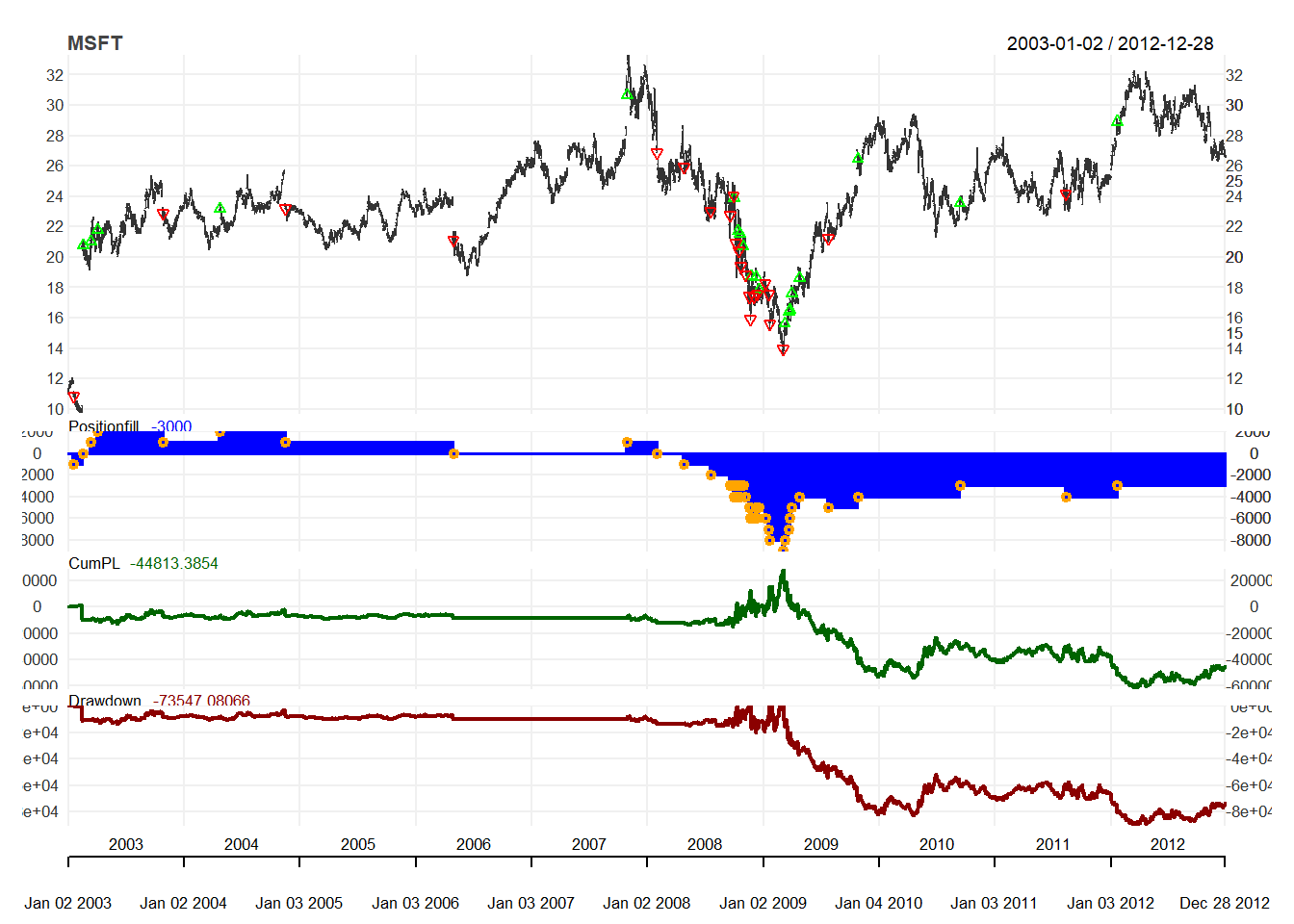
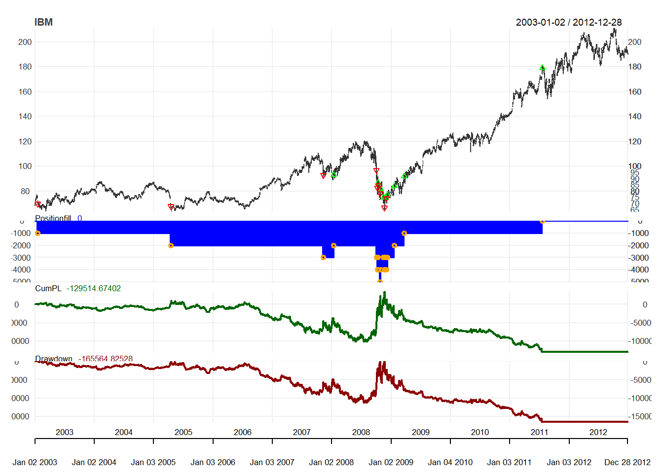
We can also look at the details of the trading statistics of trading strategies such as the number for trades, and profitability of trades.
tstats <- tradeStats(portfolio.st)
t(tstats) #transpose tstats
## IBM MSFT
## Portfolio "filter" "filter"
## Symbol "IBM" "MSFT"
## Num.Txns "18" "43"
## Num.Trades " 9" "20"
## Net.Trading.PL "-129514.67" " -44813.39"
## Avg.Trade.PL "-14390.519" " -1240.858"
## Med.Trade.PL "-3391.6402" " 637.4789"
## Largest.Winner "7730.306" "2144.921"
## Largest.Loser "-101634.719" " -9929.288"
## Gross.Profits "12637.14" "13124.34"
## Gross.Losses "-142151.81" " -37941.49"
## Std.Dev.Trade.PL "33664.545" " 3795.541"
## Std.Err.Trade.PL "11221.5151" " 848.7089"
## Percent.Positive "44.44444" "65.00000"
## Percent.Negative "55.55556" "35.00000"
## Profit.Factor "0.08889891" "0.34590998"
## Avg.Win.Trade "3159.285" "1009.565"
## Med.Win.Trade "2183.3104" " 994.9941"
## Avg.Losing.Trade "-28430.363" " -5420.214"
## Med.Losing.Trade "-14480.231" " -5107.931"
## Avg.Daily.PL "-14390.519" " -1240.858"
## Med.Daily.PL "-3391.6402" " 637.4789"
## Std.Dev.Daily.PL "33664.545" " 3795.541"
## Std.Err.Daily.PL "11221.5151" " 848.7089"
## Ann.Sharpe "-6.785846" "-5.189775"
## Max.Drawdown "-167086.24" " -90367.58"
## Profit.To.Max.Draw "-0.7751367" "-0.4959011"
## Avg.WinLoss.Ratio "0.1111236" "0.1862592"
## Med.WinLoss.Ratio "0.1507787" "0.1947940"
## Max.Equity "36050.15" "28733.70"
## Min.Equity "-131036.09" " -61633.88"
## End.Equity "-129514.67" " -44813.39"Then we can evaluate the performance using PerfomanceAnalytics package to see how is the return of the trading strategy.
rets <- PortfReturns(Account = account.st)
rownames(rets) <- NULL
tab <- table.Arbitrary(rets,
                       metrics=c(
                         "Return.cumulative",
                         "Return.annualized",
                         "SharpeRatio.annualized",
                         "CalmarRatio"),
                       metricsNames=c(
                         "Cumulative Return",
                         "Annualized Return",
                         "Annualized Sharpe Ratio",
                         "Calmar Ratio"))
tab
## IBM.DailyEqPL MSFT.DailyEqPL
## Cumulative Return -0.8776990 -0.48531918
## Annualized Return -0.1897894 -0.06436181
## Annualized Sharpe Ratio -0.4801946 -0.31095346
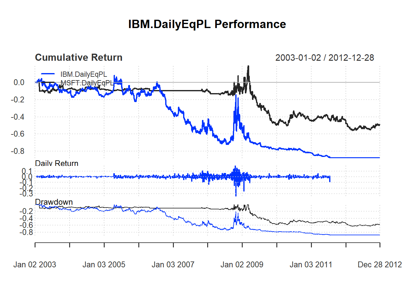
## Calmar Ratio -0.2135370 -0.10181890We can visualize the performance of the trading rule
charts.PerformanceSummary(rets, colorset = bluefocus)