23  Bayesian Simple Linear Regression Model

Regression is one of the most widely used statistical techniques for modeling relationships between variables. We will now consider a Bayesian treatment of simple linear regression. We’ll use the following example throughout.

Percent body fat (PBF, total mass of fat divided by total body mass) is an indicator of physical fitness level, but it is difficult to measure accurately. Body mass index (BMI), which is easily computed based on height and weight (\(\text{BMI} = \frac{\text{weight in kg}}{\text{(height in m)}^2}\)), is another commonly used measure¹. What is the relationship between BMI and percent body fat? How can we use a person’s BMI to estimate their percent body fat?

We’ll fit a Bayesian model for predicting percent body fat from BMI using data on a nationally representative sample of 2157 U.S. males from the National Health and Nutrition Examination Survey (NHANES).

Example 23.1 Consider the assumptions of a Bayesian simple linear regression model for predicting percent body fat from BMI.

1. What are the assumptions of the simple linear regression model? (There are many different regression models. We’re referring to the one that is usually the first one you see in introductory statistics. Sometimes the assumptions are summarized with the acronym “LINE”.)
   
   
   
   
   

2. What are the parameters in the model? That is, what do we need to put a prior distribution on (in order to eventually get a posterior distribution given sample data)? What do the parameters represent in context?
   
   
   
   
   

3. Suggest a prior distribution. Explain your reasoning.
   
   
   
   
   

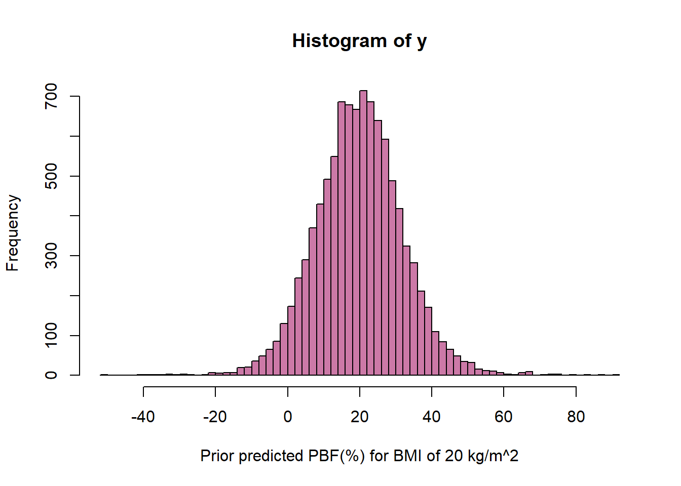
4. Describe in full detail how you would simulate the prior predictive distribution of percent body fat for males with a BMI of 20.
   
   
   
   
   
   

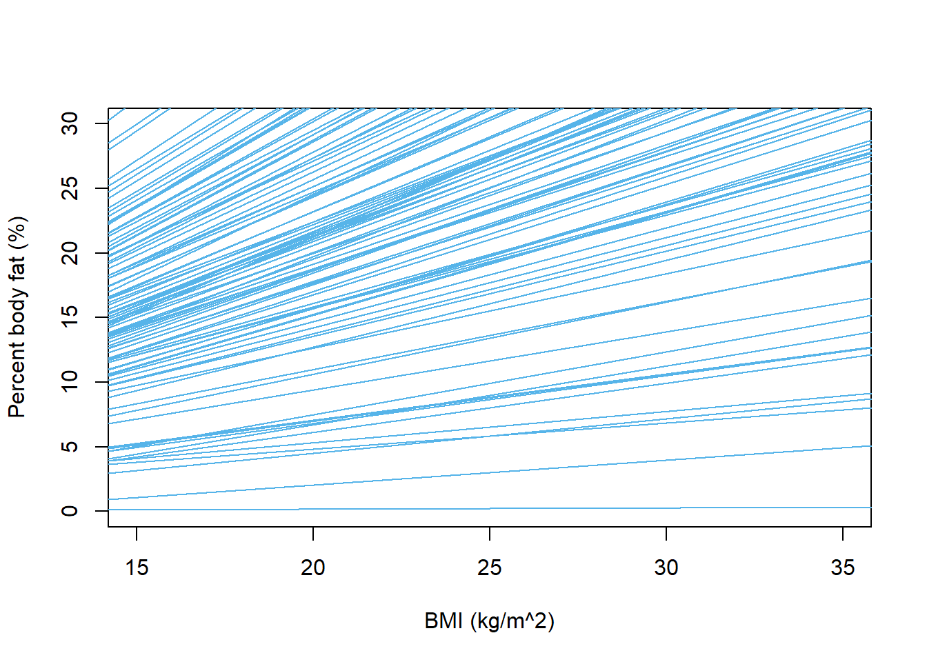
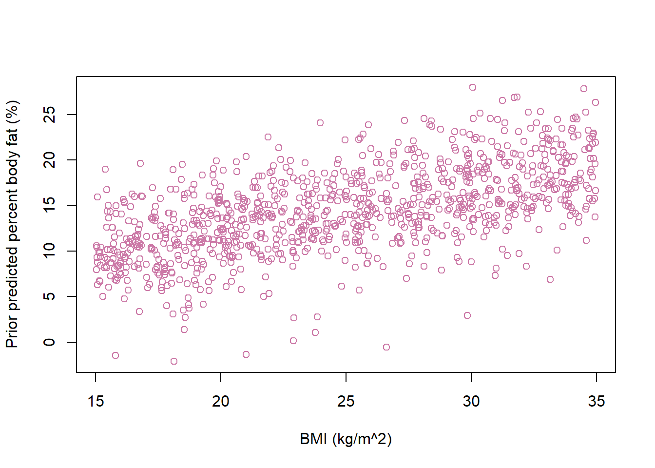
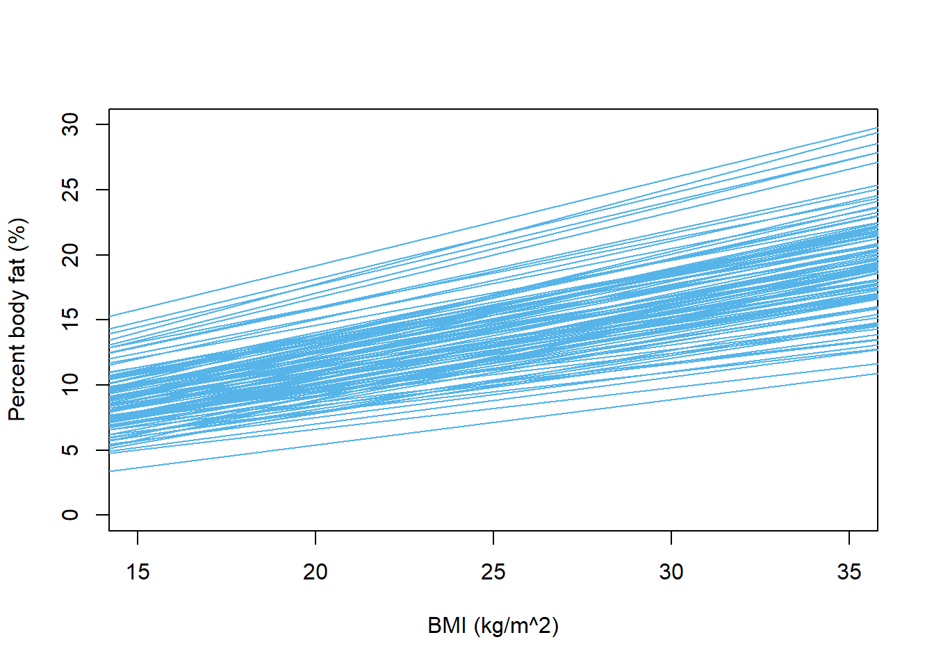
5. Simulate the prior predictive distribution of percent body fat for a range of BMI values. Do the distributions seem reasonable? If not, experiment with different priors until you find one that produces a reasonable prior predictive distribution.
   
   
   
   
   

• Consider data on a numerical response variable \(y\) and a numerical explanatory (or predictor) variable \(x\). A simple linear regression model of \(y\) on \(x\) assumes:
  • Linearity: the conditional mean of \(y\) is linear in \(x\); for some slope \(\beta_1\) and intercept \(\beta_0\): \[ \text{E}(y|x) = \beta_0 + \beta_1 x \]
  • Independence: \(y_1,\ldots, y_n\) are independent²
  • Normality: for each \(x\), the conditional distribution of \(y\) given \(x\) is Normal
  • Equal variance: the conditional variance of \(y\) does not depend on \(x\) \[ \text{Var}(y|x) = \sigma^2 \]
• The regression model is conditional. That is, we make assumptions about and perform inference for the conditional distribution of the response variable \(y\) given values of the explanatory variable \(x\). Therefore, even when we technically have a sample of pairs \((x_i,y_i)\) from a bivariate distribution, we will always condition on the values of \(x\) and treat them as non-random.
• Linearity is an assumption: we assume there is some “true” population regression line \(\beta_0 + \beta_1 x\) which specifies the conditional mean of the response variable for each value of the explanatory variable.
• The above set of assumptions can be stated more compactly as \[ y_i \sim N\left( \beta_0 + \beta_1 x_i, \sigma^2\right), \text{ and } y_1, \ldots, y_n \text{ are independent} \] Equivalently, \[ y_i = \beta_0 + \beta_1 x_i + \varepsilon_i, \text{ where } \varepsilon_i, \ldots, \varepsilon_n \text{ are i.i.d. } N(0, \sigma). \]
• The parameters of the above model are \(\beta_0\), \(\beta_1\), and \(\sigma\).
• \(\sigma_y^2\) denotes the variance of the response variable \(y\) with respect to its overall mean, while \(\sigma^2\) denotes the variance of values of the response variable about the true regression line. Thus, \(\sigma^2 = (1-\rho^2)\sigma^2_y\), where \(\rho\) is the population correlation between the explanatory and response variables.

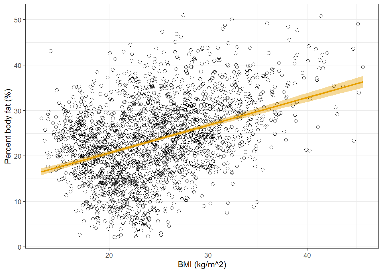
Example 23.2 Section 23.1.3 summarizes the sample data. Before fitting a Bayesian model, we’ll examine the usual frequentist results.

1. Find and interpret the slope of the fitted regression line.
   
   
   
   
   

2. Find and interpret a 95% confidence interval for the slope of the regression line. (How do you interpret 95% confidence?)
   
   
   
   
   

3. Find the equation of the fitted regression line.
   
   
   
   
   

4. Find and interpret the fitted value for men with a BMI of 20 kg/m².
   
   
   
   
   

5. Find and interpret a 95% confidence interval based on the fitted value for men with a BMI of 20 kg/m².
   
   
   
   
   

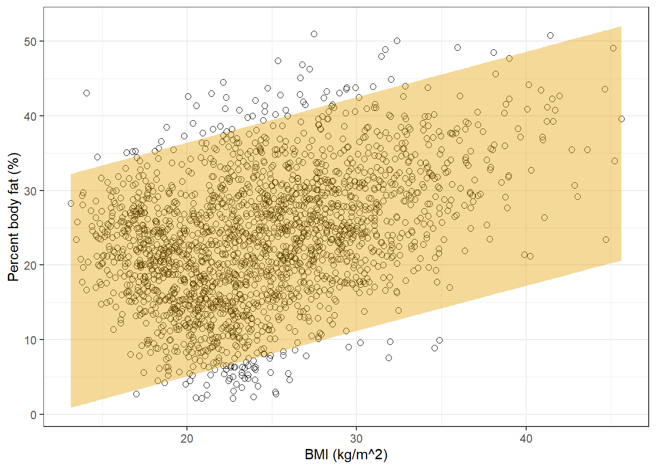
6. Find and interpret a point estimate of \(\sigma\).
   
   
   
   
   
   

7. Find and interpret a 95% prediction interval for men with a BMI of 20 kg/m².
   
   
   
   
   

Example 23.3 Now we’ll fit a Bayesian model and find the posterior distribution.

1. Suppose there are just two observations of (BMI, PBF): (15, 20) and (40, 30). How would you compute the likelihood?
   
   
   
   
   

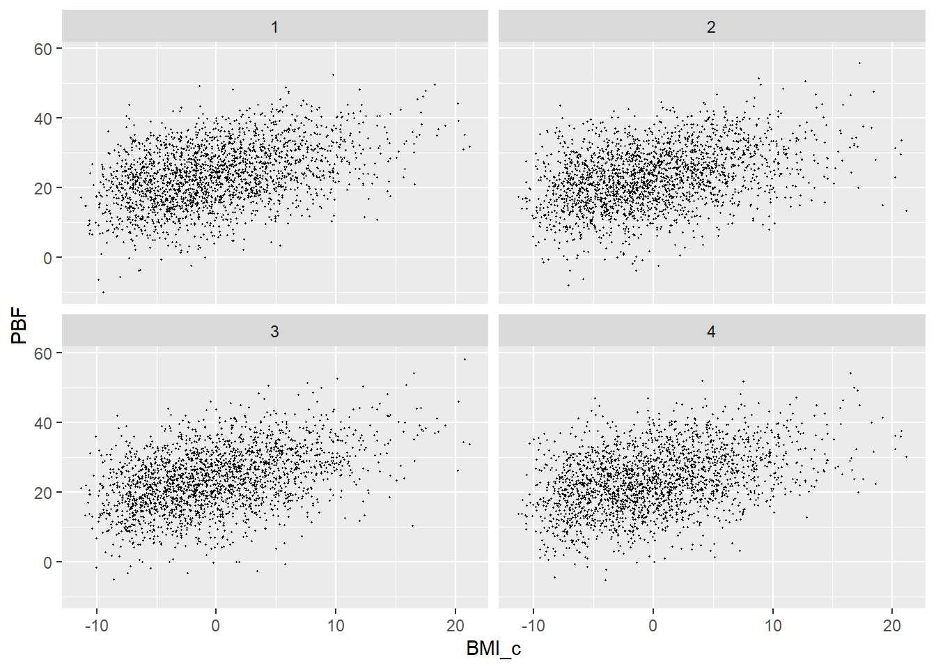
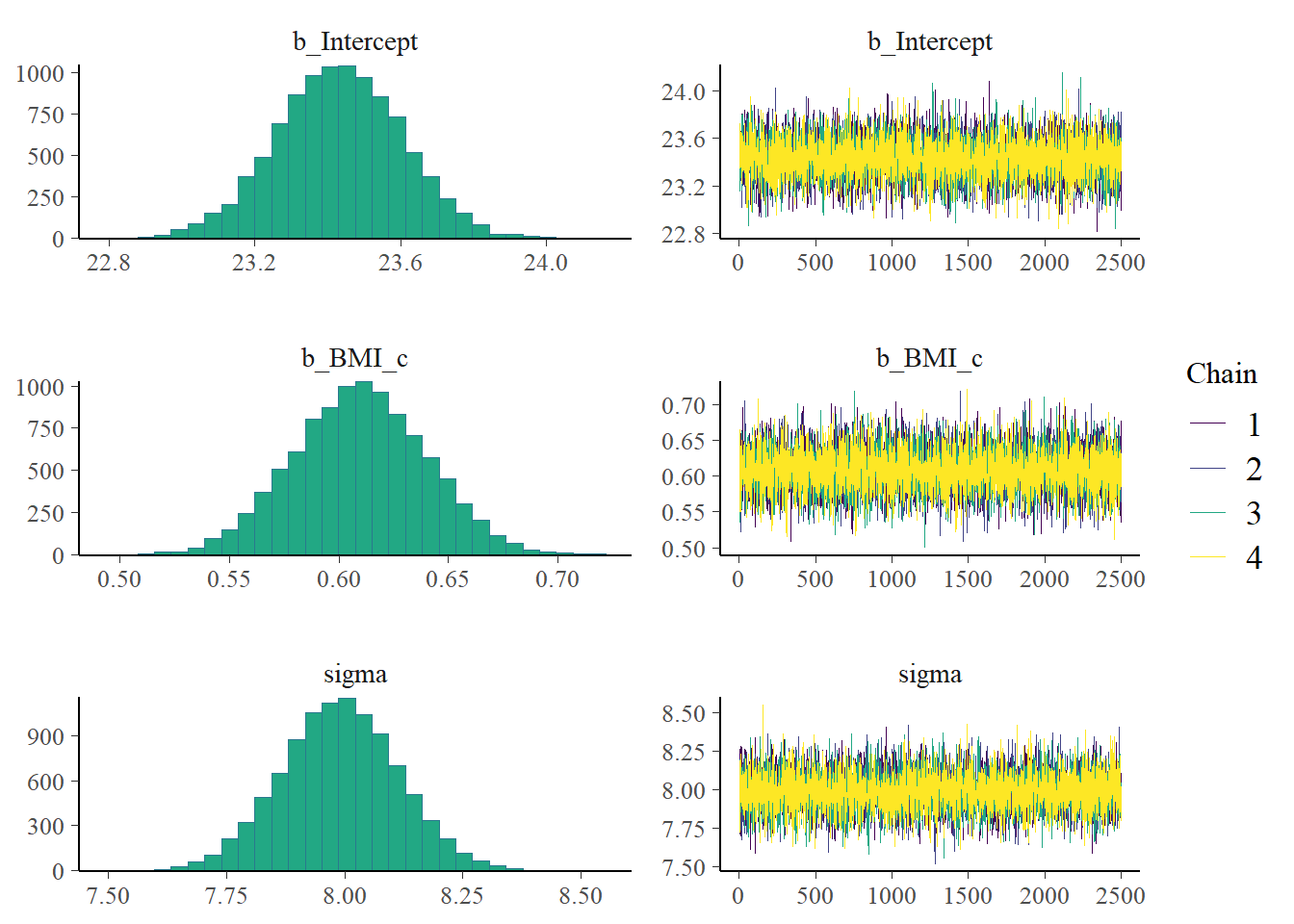
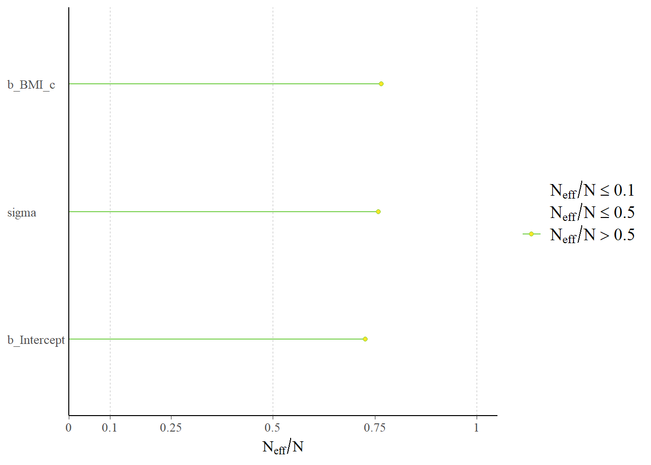
2. Use brms to fit the model to the full sample data. Run some diagnostic checks; does the MCMC algorithm seem to be working efficiently?
   
   
   
   
   

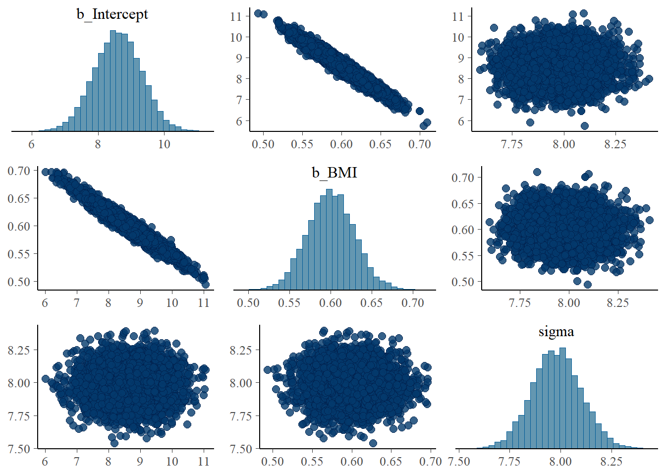
3. Inspect the joint posterior distribution of \(\beta_0\) and \(\beta_1\). What do you notice? Why do you think this happens?
   
   
   
   
   

4. Now suppose we replace BMI (\(x\)) with its centered version (\(x - \bar{x}\)). What does the parameter \(\beta_0\) represent in this model? Suggest a prior distribution for \(\beta_0\) (considering it in isolation).
   
   
   
   
   

5. Use brms to fit the model using centered BMI as the explanatory variable. Inspect the joint posterior distribution of \(\beta_0\) and \(\beta_1\). What do you notice? Why do you think this happens?
   
   
   
   
   

Example 23.4 Now we’ll summarize and report conclusions based on the posterior distribution, using the model with centered BMI.

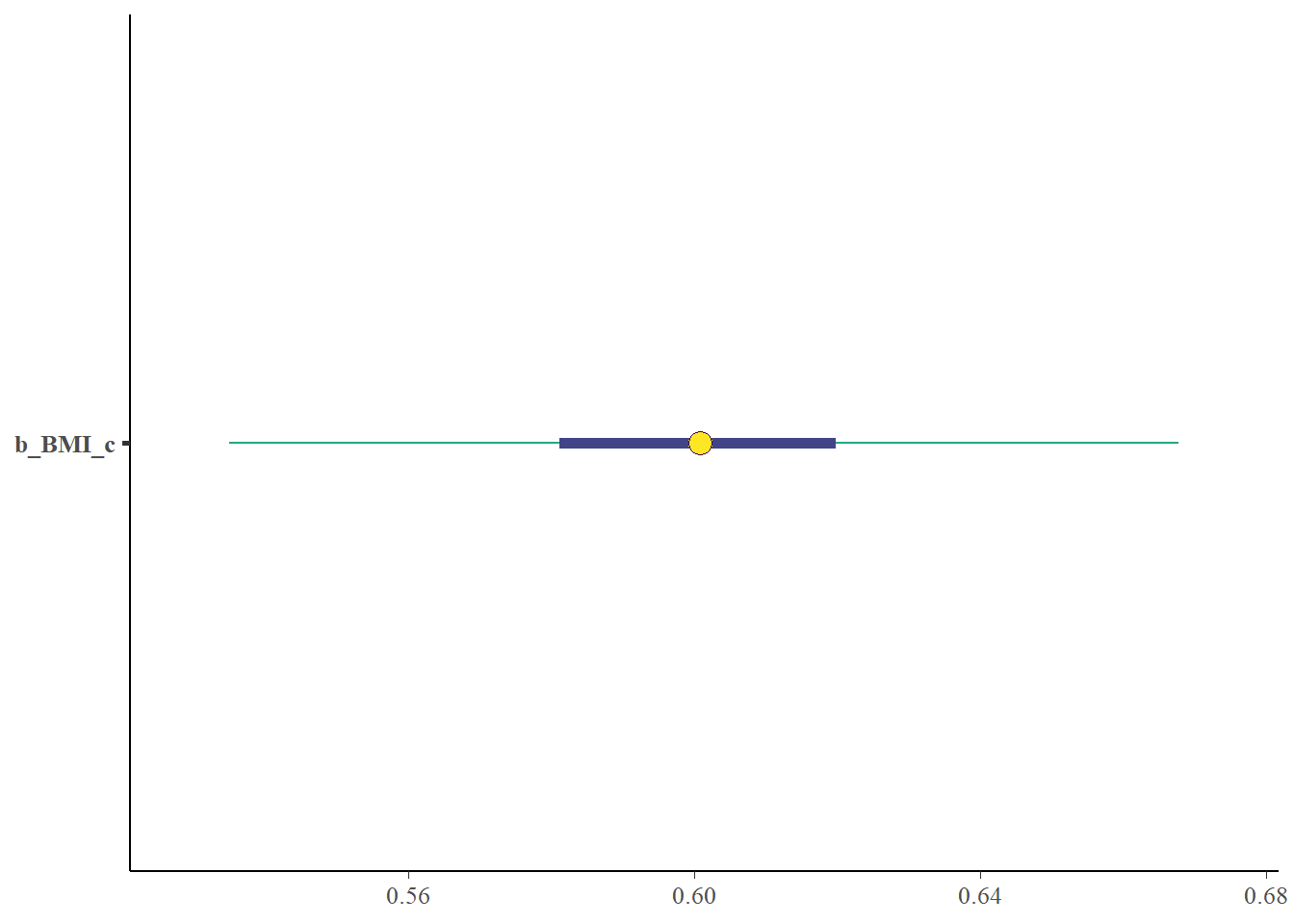
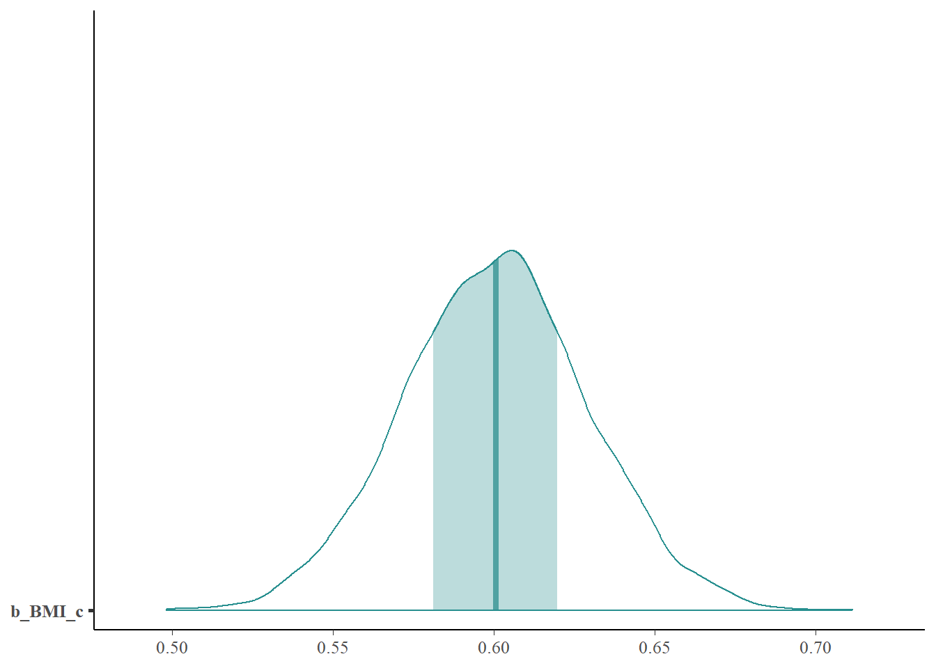
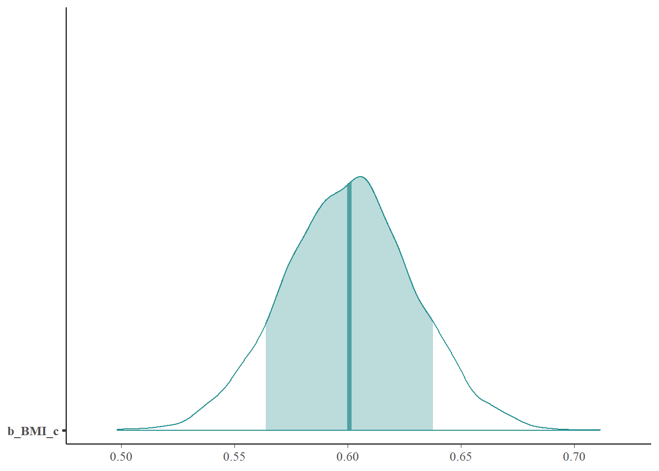
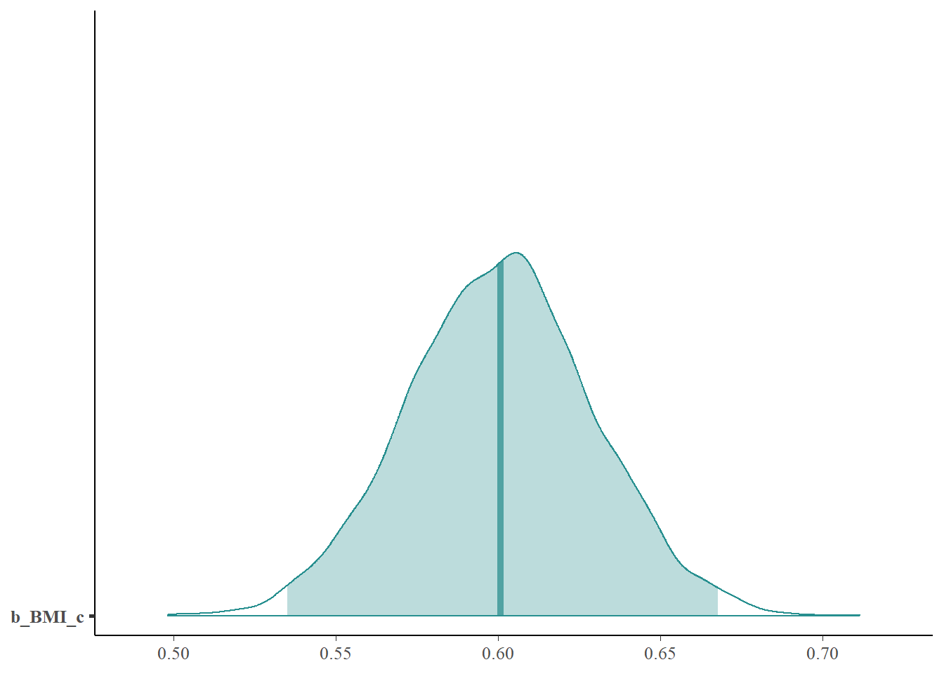
1. Describe the posterior distribution of \(\beta_1\). Find and interpret 50%, 80%, and 98% posterior credible intervals for \(\beta_1\).
   
   
   
   
   

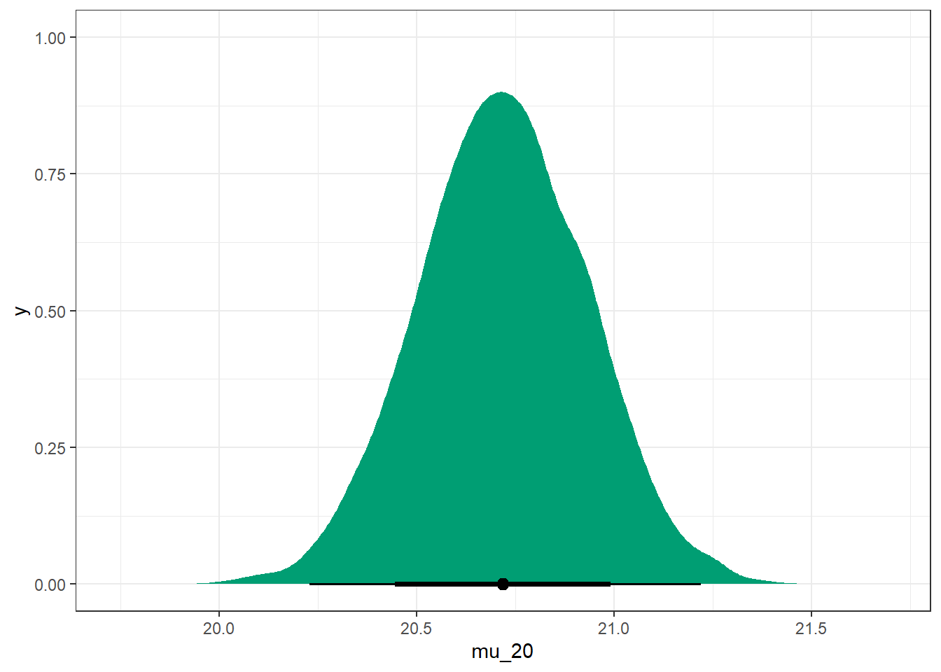
2. What does the parameter \(\mu_{20} = \beta_0 + \beta_1(20 -\bar{x})\) represent in context? Explain how you could approximate the posterior distribution of \(\mu_{20}\). Then approximate the posterior distribution, describe it, and find and interpret a 98% posterior credible interval for \(\mu_{20}\).
   
   
   
   
   

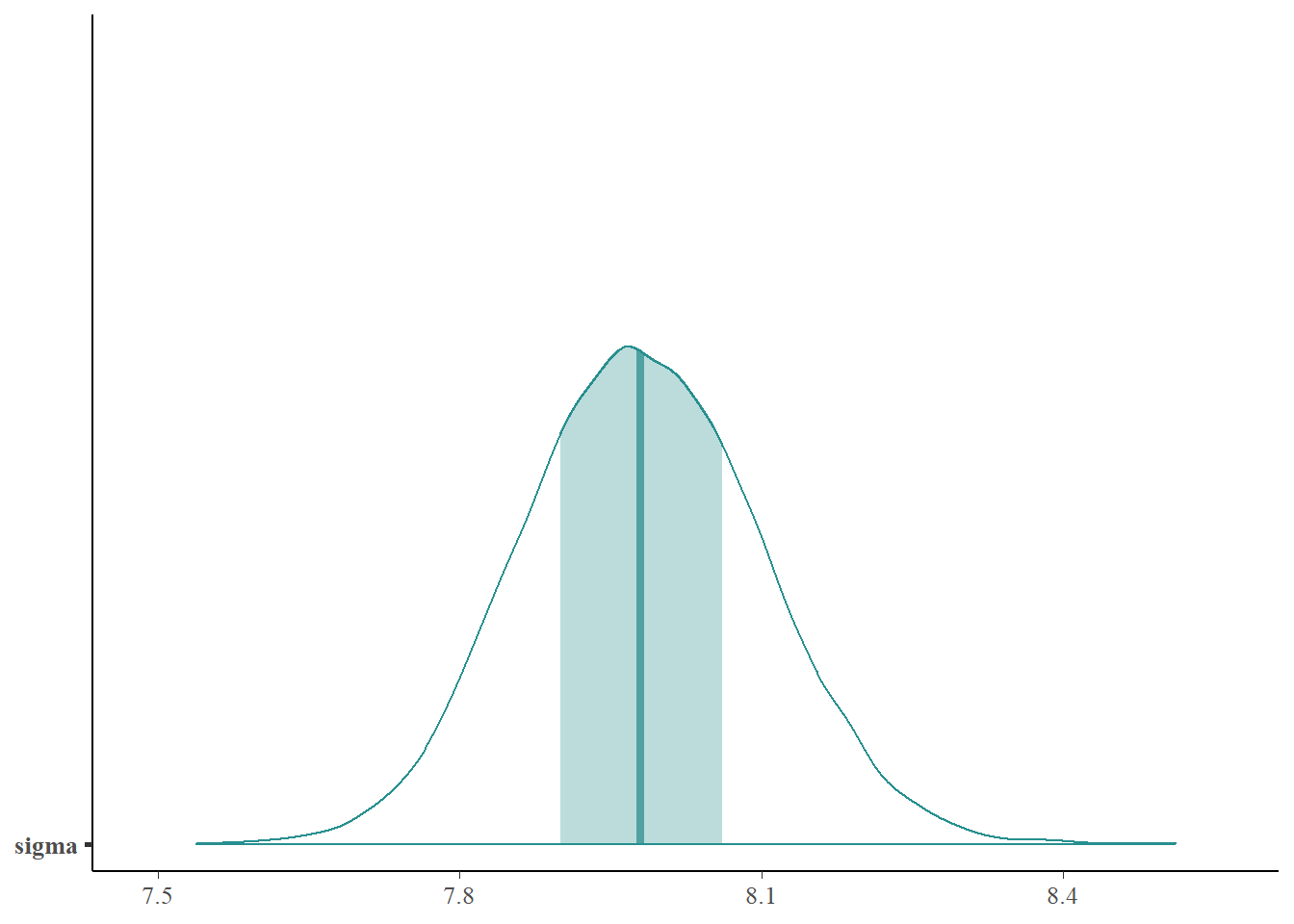
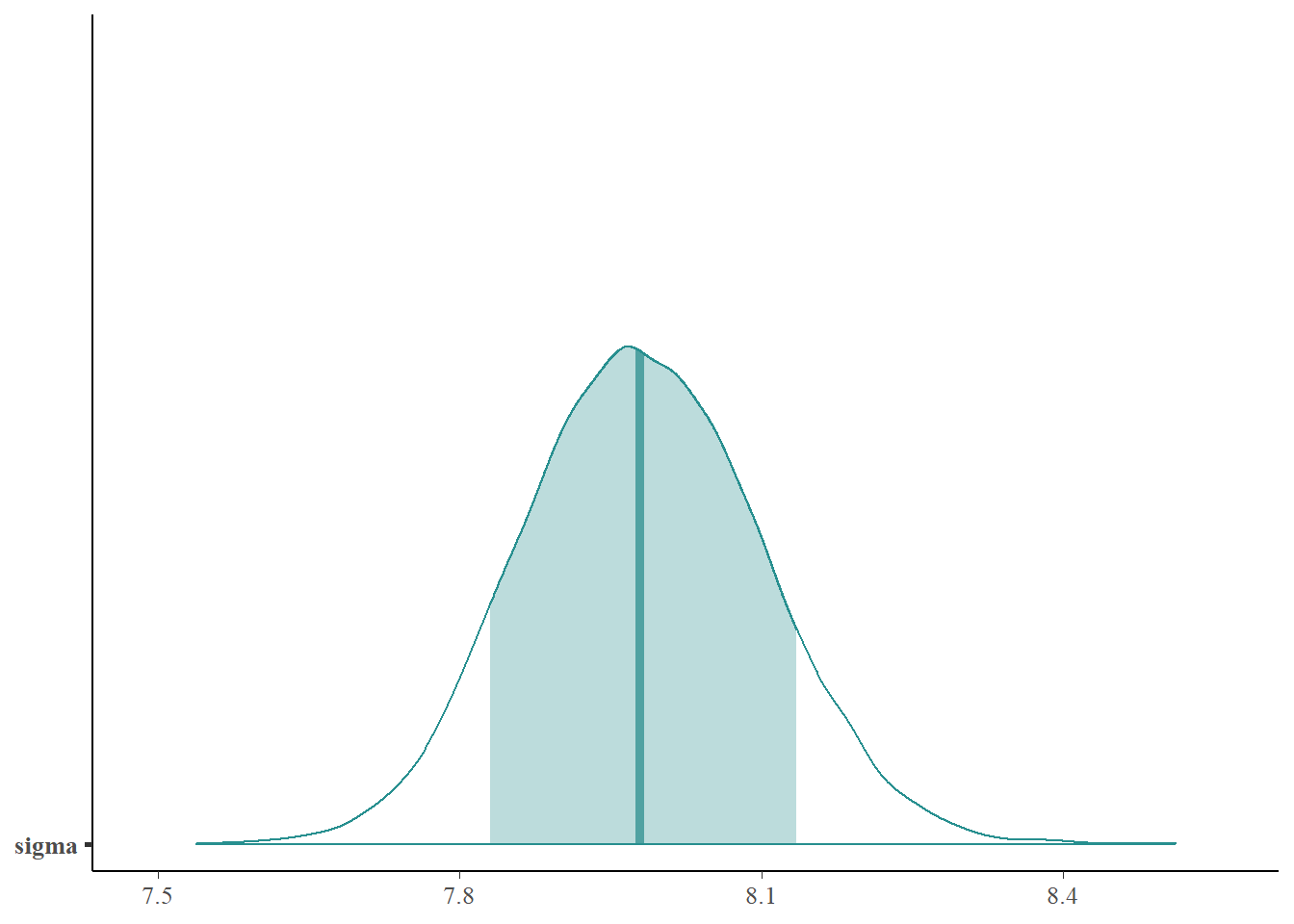
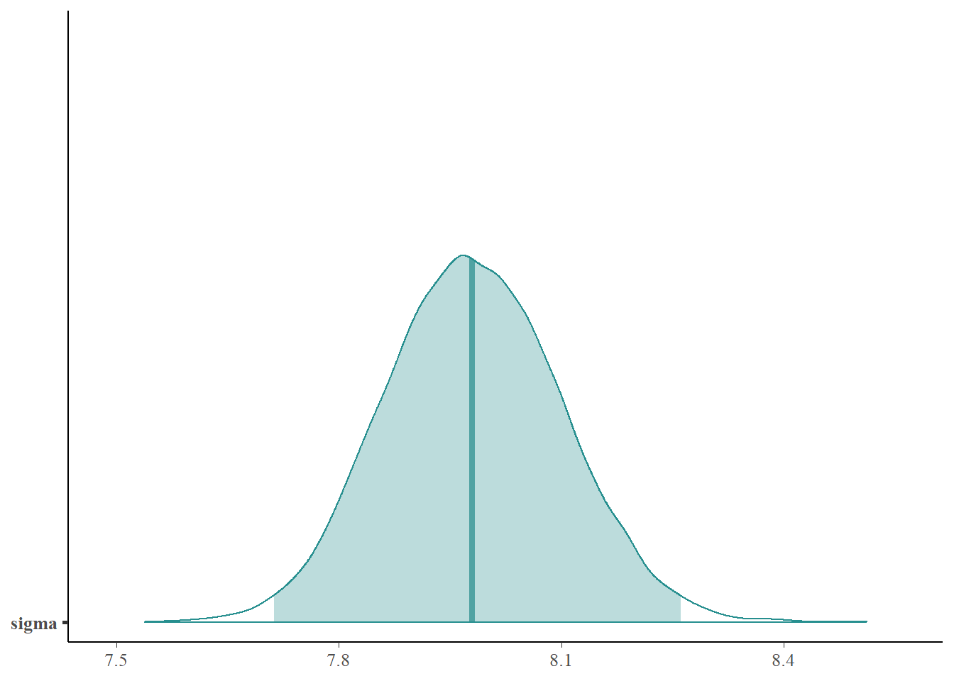
3. Describe the posterior distribution of \(\sigma\). Find and interpret 50%, 80%, and 98% posterior credible intervals for \(\sigma\).
   
   
   
   
   

4. Compare the results of the Bayesian and frequentist analyses. How are they similar? How are they different?
   
   
   
   
   

Example 23.5 Now we’ll use the fitted model to predict percent body fat.

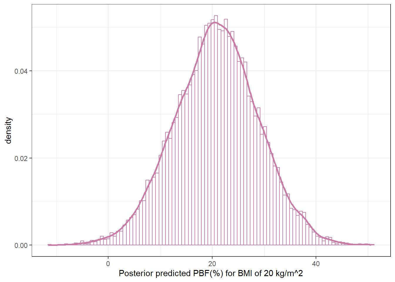
1. Explain how you could approximate the posterior predictive distribution of percent body fat for men with a BMI of 20 kg/m².
   
   
   
   
   

2. Find and interpret a 95% posterior prediction interval for men with a BMI of 20 kg/m².
   
   
   
   
   

3. Compare the 95% posterior prediction interval with the corresponding frequentist 95% prediction interval. How are they similar? How are they different?
   
   
   
   
   

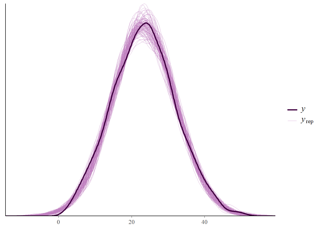
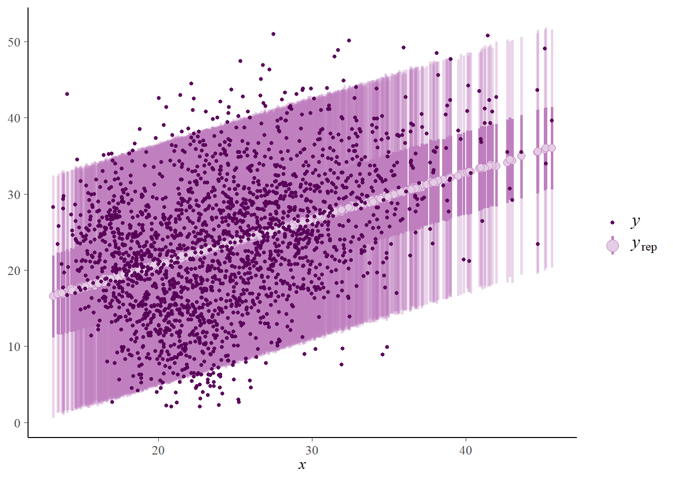
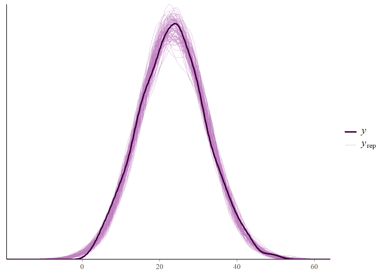
4. Suggest how you could perform a posterior predictive check. Then use software to perform the check. Does the model seem reasonable based on the data?
   
   
   
   
   

• There are a number of ways the assumptions of the simple linear regression model could be revised.
• We could assume the mean of \(y\) changes with \(x\) is a non-linear way (e.g., quadratic).
• We could assume distributions other than Normal in the likelihood. For example, we could assume a \(t\)-distribution if outliers were an issue.
• We could assume the conditional variance of \(y\) also changes with \(x\).
• We could include multiple explanatory variables \(x\).
• Each of the above would be a change in the likelihood, perhaps introducing additional parameters.

Example 23.6 Now we’ll investigate sensitivity of the results to choice of prior. Rerun the model (using centered BMI) but let brms choose the prior. Compare the results of the two Bayesian models; are the results very sensitive to the choice of prior?

23.1 Notes

23.1.1 Prior predictive tuning

• We’ll start with a prior distribution under which \(\beta_0\), \(\beta_1\), and \(\sigma\) are independent.
• A quick Google search reveals that for men percent body fat ranges from about 6% to 30%, and BMI ranges from about 15 to 35 kg/m².
• The overall range of percent body fat is about 6% to 30%, but we would expect less variability among men of the same BMI. If we assume percent body fat varies by about 5 percentage points among men of the same BMI, we can choose a prior for \(\sigma\) that has a mean of 5, say Exponential(1/5) (to reflect \(\sigma>0\)).
• We expect a positive association between percent body fat and BMI, so we want a prior for \(\beta_1\) that places most of its credibility on positive values. Disregarding measurement units, the two variables take values on fairly similar numerical scales (6 to 30, 15 to 35). For the slope \(\beta_1\), we might assume a Normal prior with a mean of 1 and a standard deviation of 0.5 (to keep most of the credibility on positive values, reflecting prior belief in positive association).
• The intercept \(\beta_0\), in principle, represents the percent body fat for a man with a BMI of 0, so we might assume a Normal prior with a mean of 0 and a standard deviation of 1 (to put most of the prior credibility near 0). (We’ll see another way to think about this parameter soon.) In summary, our prior distribution on the parameters \((\beta_0, \beta_1, \sigma)\) assumes
  • \(\beta_0\), \(\beta_1\), and \(\sigma\) are independent
  • \(\sigma \sim\) Exponential(1/5)
  • \(\beta_1\sim\) Normal(1, 0.5)
  • \(\beta_0\sim\) Normal(0, 1)

Prior predictive distribution for BMI of 20

n_rep = 10000

# value of x
x = 20

# simulate parameters from prior distribution
beta0 = rnorm(n_rep, 0, 1)
beta1 = rnorm(n_rep, 1, 0.5)
sigma = rexp(n_rep, 1 / 5)

# simulate values of percent body fat based on assumptions of regression model
y = rnorm(n_rep, beta0 + beta1 * x, sigma)

hist(y, xlab = "Prior predicted PBF(%) for BMI of 20 kg/m^2",
     breaks = 100,
     col = bayes_col["prior_predict"])

Prior predictive distribution for many values of BMI

n_rep = 1000

# a range of values of x
x = runif(n_rep, 15, 35)

# simulate parameters from prior distribution
beta0 = rnorm(n_rep, 0, 1)
beta1 = rnorm(n_rep, 1, 0.5)
sigma = rexp(n_rep, 1 / 5)

# simulate values of percent body fat based on assumptions of regression model
y = rnorm(n_rep, beta0 + beta1 * x, sigma)

# scatter plot or prior predicted values
plot(x, y,
     xlab = "BMI (kg/m^2)", ylab = "Prior predicted percent body fat (%)",
     col = bayes_col["prior_predict"])

What regression lines might look like according to prior distribution

# number of lines to plot
n_lines = 100

# blank scatterplot - just set the plot area and scale
plot(x, y, xlab = "BMI (kg/m^2)", ylab = "Percent body fat (%)", type = "n",
 xlim = c(15, 35),
 ylim = c(0, 30))

# plot each of the simulated lines
# using slope and intercept simulated from prior distribution
for (l in 1:n_lines){
  abline(beta0[l], beta1[l], col = bayes_col["prior"], lwd = 1)
}

23.1.2 Prior predictive distribution

After some tuning, our prior distribution on the parameters \((\beta_0, \beta_1, \sigma)\) assumes

• \(\beta_0\), \(\beta_1\), and \(\sigma\) are independent
• \(\sigma \sim\) Exponential(1/1.5)
• \(\beta_1\sim\) Normal(0.5, 0.1)
• \(\beta_0\sim\) Normal(2, 2)

Prior predictive distributions

n_rep = 1000

# a range of values of x
x = runif(n_rep, 15, 35)

# simulate parameters from prior distribution
beta0 = rnorm(n_rep, 2, 2)
beta1 = rnorm(n_rep, 0.5, 0.1)
sigma = rexp(n_rep, 1 / 1.5)

# simulate values of percent body fat based on assumptions of regression model
y = rnorm(n_rep, beta0 + beta1 * x, sigma)

# scatter plot or prior predicted values
plot(x, y,
     xlab = "BMI (kg/m^2)", ylab = "Prior predicted percent body fat (%)",
     col = bayes_col["prior_predict"])

# number of lines to plot
n_lines = 100

# blank scatterplot - just set the plot area and scale
plot(x, y, xlab = "BMI (kg/m^2)", ylab = "Percent body fat (%)", type = "n",
 xlim = c(15, 35),
 ylim = c(0, 30))

# plot each of the simulated lines
# using slope and intercept simulated from prior distribution
for (l in 1:n_lines){
  abline(beta0[l], beta1[l], col = bayes_col["prior"], lwd = 1)
}

23.1.3 Sample data

data = read_csv("nhanes_males.csv")

Rows: 2157 Columns: 2
── Column specification ────────────────────────────────────────────────────────
Delimiter: ","
dbl (2): BMI, PBF

ℹ Use `spec()` to retrieve the full column specification for this data.
ℹ Specify the column types or set `show_col_types = FALSE` to quiet this message.

data |> head() |> kbl() |> kable_styling()

BMI	PBF
20.65	13.1
21.46	31.9
26.76	24.9
26.41	23.5
15.46	25.2
23.90	7.2

c(summary(data$BMI), SD = sd(data$BMI))

     Min.   1st Qu.    Median      Mean   3rd Qu.      Max.        SD 
13.140000 20.150000 23.800000 24.449907 28.100000 45.610000  5.688115 

c(summary(data$PBF), SD = sd(data$PBF))

     Min.   1st Qu.    Median      Mean   3rd Qu.      Max.        SD 
 2.100000 17.400000 23.500000 23.432313 29.200000 51.000000  8.704317 

cor(data$BMI, data$PBF)

[1] 0.3981832

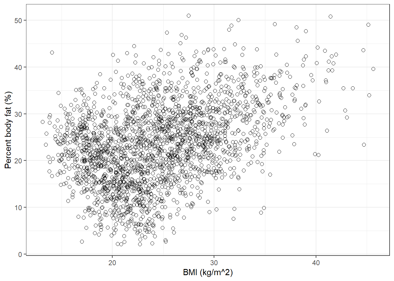
data_plot = ggplot(data, 
                   aes(x = BMI, y = PBF)) +
  geom_point(shape = 1, size = 2) +
  labs(x = "BMI (kg/m^2)",
       y = "Percent body fat (%)") +
  theme_bw()

data_plot

23.1.4 Frequentist results

freq = lm(PBF ~ BMI, data)

summary(freq)

Call:
lm(formula = PBF ~ BMI, data = data)

Residuals:
     Min       1Q   Median       3Q      Max 
-21.2198  -5.5169   0.2299   5.4232  26.0046 

Coefficients:
            Estimate Std. Error t value Pr(>|t|)    
(Intercept)  8.53437    0.75906   11.24   <2e-16 ***
BMI          0.60933    0.03024   20.15   <2e-16 ***
---
Signif. codes:  0 '***' 0.001 '**' 0.01 '*' 0.05 '.' 0.1 ' ' 1

Residual standard error: 7.986 on 2155 degrees of freedom
Multiple R-squared:  0.1585,    Adjusted R-squared:  0.1582 
F-statistic: 406.1 on 1 and 2155 DF,  p-value: < 2.2e-16

Confidence interval for mean response

x_new = data.frame(BMI = 20)

predict(freq, newdata = x_new, interval = "confidence", se.fit = TRUE)

$fit
       fit      lwr      upr
1 20.72087 20.29268 21.14907

$se.fit
[1] 0.2183474

$df
[1] 2155

$residual.scale
[1] 7.986374

data_plot +
  geom_smooth(method = lm,
              col = bayes_col["likelihood"],
              fill = bayes_col["likelihood"])

Prediction intervals

x_new = data.frame(BMI = 20)

predict(freq, newdata = x_new, interval = "prediction")

       fit      lwr      upr
1 20.72087 5.053218 36.38853

predictions <- predict(freq, interval = "predict")

data |>
  cbind(predictions) |>
  ggplot(aes(x = BMI, y = PBF)) +
  geom_point(shape = 1, size = 2) +
  geom_ribbon(aes(ymin = lwr, ymax = upr),
              fill = bayes_col["likelihood"], alpha = 0.4) +
  labs(x = "BMI (kg/m^2)",
       y = "Percent body fat (%)") +
  theme_bw()

23.1.5 Posterior distribution

library(brms)

Loading required package: Rcpp

Loading 'brms' package (version 2.21.0). Useful instructions
can be found by typing help('brms'). A more detailed introduction
to the package is available through vignette('brms_overview').

Attaching package: 'brms'

The following object is masked from 'package:stats':

    ar

library(tidybayes)

Attaching package: 'tidybayes'

The following objects are masked from 'package:brms':

    dstudent_t, pstudent_t, qstudent_t, rstudent_t

library(bayesplot)

This is bayesplot version 1.11.1

- Online documentation and vignettes at mc-stan.org/bayesplot

- bayesplot theme set to bayesplot::theme_default()

   * Does _not_ affect other ggplot2 plots

   * See ?bayesplot_theme_set for details on theme setting

Attaching package: 'bayesplot'

The following object is masked from 'package:brms':

    rhat

fit <- brm(data = data,
           family = gaussian(),
           PBF ~ 1 + BMI,
           prior = c(prior(normal(2, 2), class = Intercept),
                     prior(normal(0.5, 0.1), class = b),
                     prior(exponential(0.667), class = sigma)),
           iter = 3500,
           warmup = 1000,
           chains = 4,
           refresh = 0)

Compiling Stan program...

Start sampling

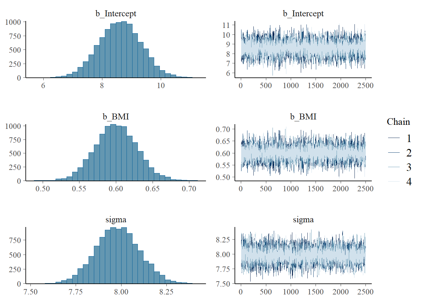
summary(fit)

 Family: gaussian 
  Links: mu = identity; sigma = identity 
Formula: PBF ~ 1 + BMI 
   Data: data (Number of observations: 2157) 
  Draws: 4 chains, each with iter = 3500; warmup = 1000; thin = 1;
         total post-warmup draws = 10000

Regression Coefficients:
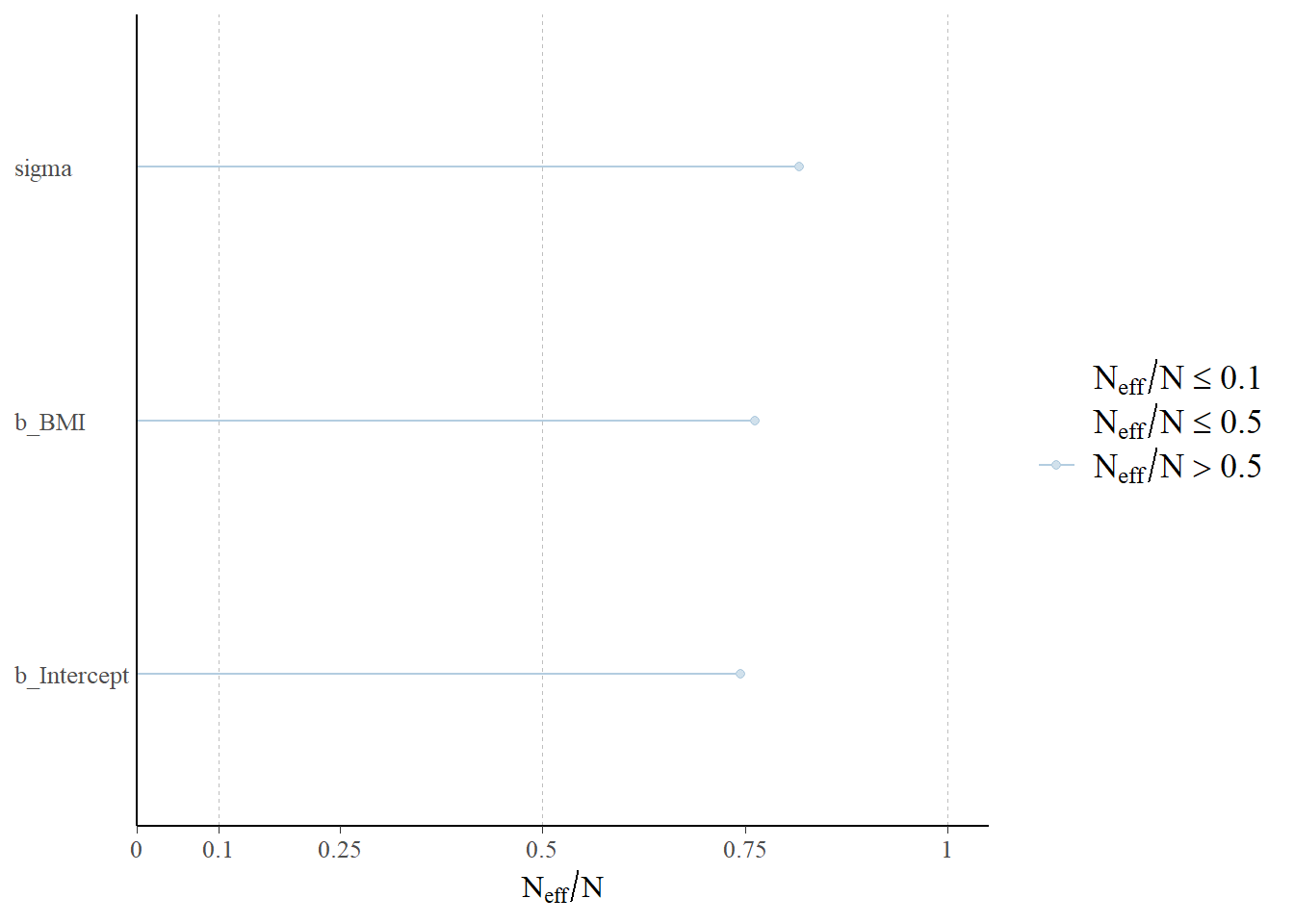
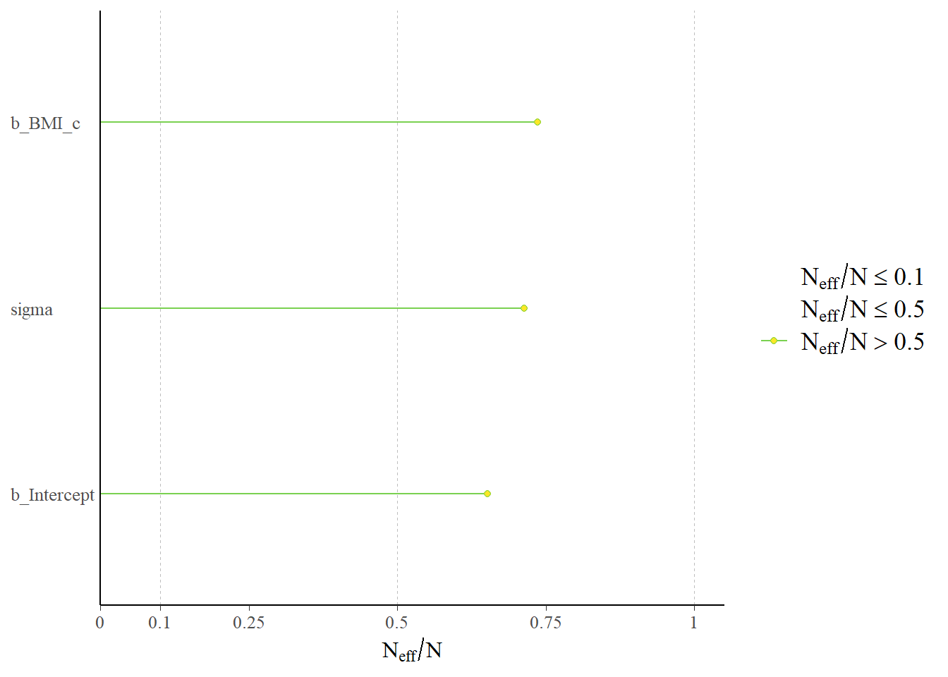
          Estimate Est.Error l-95% CI u-95% CI Rhat Bulk_ESS Tail_ESS
Intercept     8.60      0.72     7.20     9.99 1.00    10059     7435
BMI           0.60      0.03     0.55     0.66 1.00    10239     7616

Further Distributional Parameters:
      Estimate Est.Error l-95% CI u-95% CI Rhat Bulk_ESS Tail_ESS
sigma     7.98      0.12     7.75     8.22 1.00    10922     8170

Draws were sampled using sampling(NUTS). For each parameter, Bulk_ESS
and Tail_ESS are effective sample size measures, and Rhat is the potential
scale reduction factor on split chains (at convergence, Rhat = 1).

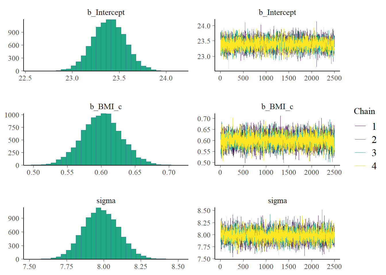
plot(fit)

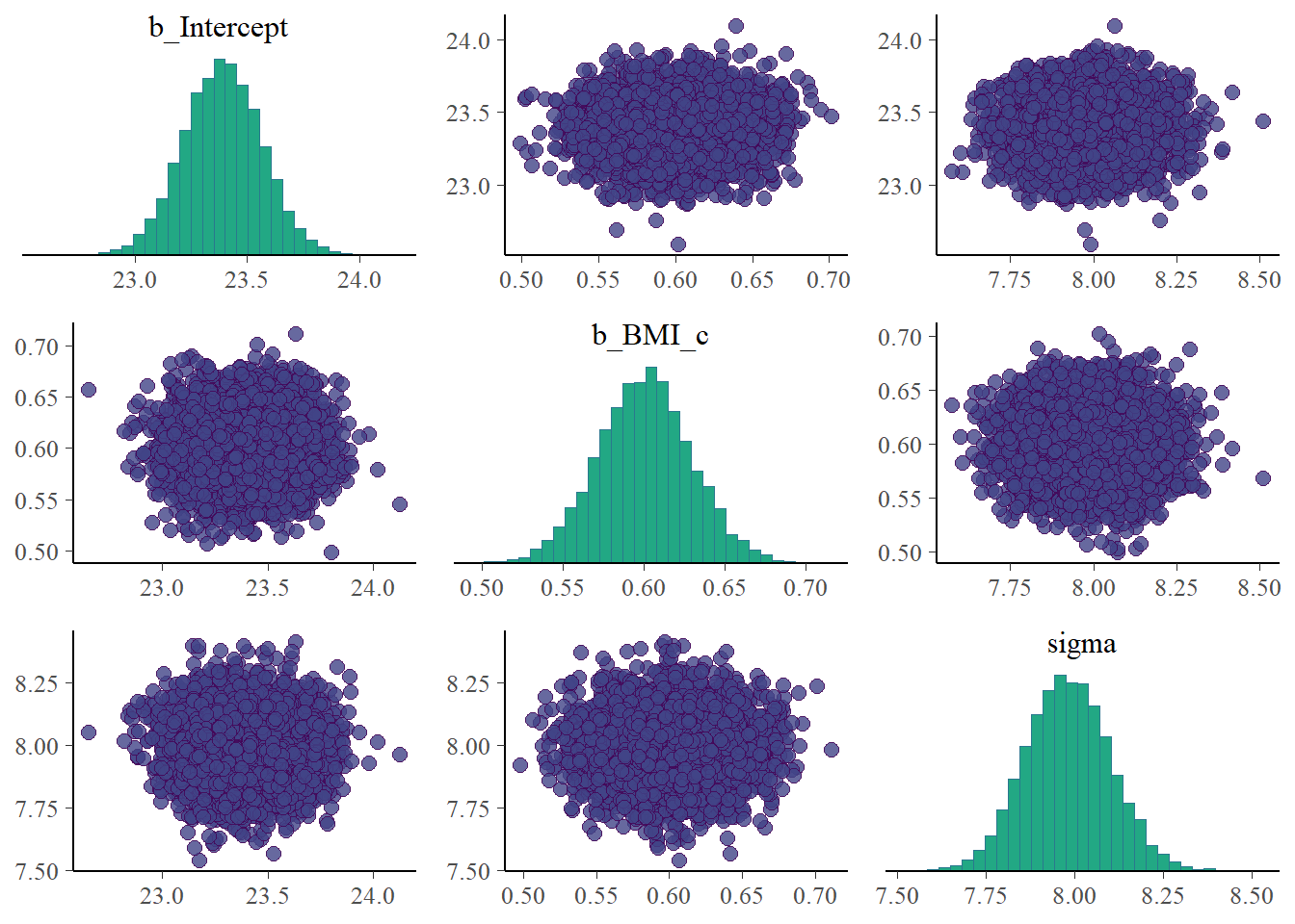
pairs(fit)

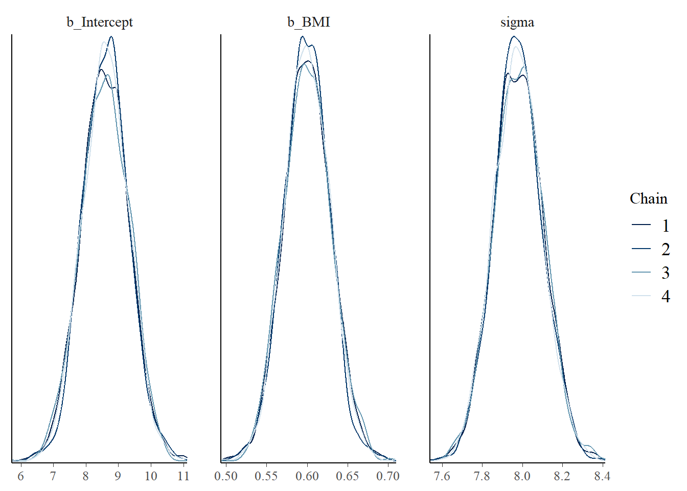
mcmc_dens_overlay(fit, pars = vars(b_Intercept, b_BMI, sigma))

neff_ratio(fit)[c("b_Intercept", "b_BMI", "sigma")]

b_Intercept       b_BMI       sigma 
  0.7435396   0.7615754   0.8170061 

neff_ratio(fit)[c("b_Intercept", "b_BMI", "sigma")] |> 
  mcmc_neff() +
  yaxis_text(hjust = 0) 

23.1.6 Posterior distribution, model using centered BMI

data = data |>
  mutate(BMI_c = BMI - mean(BMI))

fit_c <- brm(data = data,
           family = gaussian(),
           PBF ~ 1 + BMI_c,
           prior = c(prior(normal(18, 2), class = Intercept),
                prior(normal(0.5, 0.1), class = b),
                prior(exponential(0.667), class = sigma)),
           iter = 3500,
           warmup = 1000,
           chains = 4,
           refresh = 0)

Compiling Stan program...

Start sampling

summary(fit_c)

 Family: gaussian 
  Links: mu = identity; sigma = identity 
Formula: PBF ~ 1 + BMI_c 
   Data: data (Number of observations: 2157) 
  Draws: 4 chains, each with iter = 3500; warmup = 1000; thin = 1;
         total post-warmup draws = 10000

Regression Coefficients:
          Estimate Est.Error l-95% CI u-95% CI Rhat Bulk_ESS Tail_ESS
Intercept    23.39      0.17    23.05    23.73 1.00     8456     6517
BMI_c         0.60      0.03     0.54     0.66 1.00    11548     7352

Further Distributional Parameters:
      Estimate Est.Error l-95% CI u-95% CI Rhat Bulk_ESS Tail_ESS
sigma     7.98      0.12     7.75     8.22 1.00     9201     7129

Draws were sampled using sampling(NUTS). For each parameter, Bulk_ESS
and Tail_ESS are effective sample size measures, and Rhat is the potential
scale reduction factor on split chains (at convergence, Rhat = 1).

color_scheme_set("viridis")

plot(fit_c)

pairs(fit_c)

neff_ratio(fit_c)[c("b_Intercept", "b_BMI_c", "sigma")]

b_Intercept     b_BMI_c       sigma 
  0.6516833   0.7352337   0.7128977 

neff_ratio(fit_c)[c("b_Intercept", "b_BMI_c", "sigma")] |> 
  mcmc_neff() +
  yaxis_text(hjust = 0) 

Posterior distribution of regression slope

mcmc_intervals(fit_c,
               pars = c("b_BMI_c"),
               prob = 0.5,
               prob_outer = 0.98)

color_scheme_set("teal")

mcmc_areas(fit_c,
           pars = c("b_BMI_c"),
           prob = 0.5,
           point_est = "median")
mcmc_areas(fit_c,
           pars = c("b_BMI_c"),
           prob = 0.8,
           point_est = "median")
mcmc_areas(fit_c,
           pars = c("b_BMI_c"),
           prob = 0.98,
           point_est = "median")

Posterior distribution of \(\sigma\)

mcmc_intervals(fit_c,
               pars = c("sigma"),
               prob = 0.5,
               prob_outer = 0.98)

mcmc_areas(fit_c,
           pars = c("sigma"),
           prob = 0.5,
           point_est = "median")
mcmc_areas(fit_c,
           pars = c("sigma"),
           prob = 0.8,
           point_est = "median")
mcmc_areas(fit_c,
           pars = c("sigma"),
           prob = 0.98,
           point_est = "median")

Posterior distribution of mean response

posterior_c = fit_c |>
  spread_draws(b_Intercept, b_BMI_c, sigma) |>
  mutate(mu_20 = b_Intercept + b_BMI_c * (20 - mean(data$BMI)))

posterior_c |> head(10) |> kbl() |> kable_styling()

.chain	.iteration	.draw	b_Intercept	b_BMI_c	sigma	mu_20
1	1	1	23.27824	0.5574416	8.039549	20.79768
1	2	2	23.62545	0.6372204	7.904723	20.78987
1	3	3	23.62162	0.5754227	7.939876	21.06105
1	4	4	23.12276	0.6061011	8.060678	20.42566
1	5	5	23.12524	0.6090495	8.042735	20.41503
1	6	6	23.36472	0.6317251	8.041233	20.55360
1	7	7	23.50486	0.5616251	7.953135	21.00568
1	8	8	23.73264	0.5591934	7.967661	21.24428
1	9	9	23.01671	0.6313645	7.905566	20.20720
1	10	10	23.32895	0.5444100	7.950075	20.90638

posterior_c |>
  ggplot(aes(x = mu_20)) +
  stat_halfeye(.width = c(0.80, 0.98),
               fill = bayes_col["posterior"]) +
  theme_bw()

quantile(posterior_c$mu_20, c(0.01, 0.99))

      1%      99% 
20.22745 21.21915 

23.1.7 Posterior prediction

posterior_c = posterior_c |>
  mutate(y_pred_20 = mu_20 + sigma * rnorm(nrow(posterior_c), 0, 1))

posterior_c |> head(10) |> kbl() |> kable_styling()

.chain	.iteration	.draw	b_Intercept	b_BMI_c	sigma	mu_20	y_pred_20
1	1	1	23.27824	0.5574416	8.039549	20.79768	13.92848
1	2	2	23.62545	0.6372204	7.904723	20.78987	29.75587
1	3	3	23.62162	0.5754227	7.939876	21.06105	42.44593
1	4	4	23.12276	0.6061011	8.060678	20.42566	22.45721
1	5	5	23.12524	0.6090495	8.042735	20.41503	6.98945
1	6	6	23.36472	0.6317251	8.041233	20.55360	22.91524
1	7	7	23.50486	0.5616251	7.953135	21.00568	29.02020
1	8	8	23.73264	0.5591934	7.967661	21.24428	17.71785
1	9	9	23.01671	0.6313645	7.905566	20.20720	17.87872
1	10	10	23.32895	0.5444100	7.950075	20.90638	6.83985

ggplot(posterior_c,
       aes(x = y_pred_20)) +
  geom_histogram(aes(y = after_stat(density)),
                 col = bayes_col["posterior_predict"], fill = "white", bins = 100) +
  geom_density(linewidth = 1, col = bayes_col["posterior_predict"]) +
  labs(x = "Posterior predicted PBF(%) for BMI of 20 kg/m^2") +
  theme_bw()

quantile(posterior_c$y_pred_20, c(0.025, 0.975))

     2.5%     97.5% 
 4.791813 36.748738 

predictive_interval(fit_c,
                    newdata = data.frame(BMI_c = 20 - mean(data$BMI)),
                    prob = 0.95)

         2.5%    97.5%
[1,] 4.722616 36.10427

23.1.8 Posterior predictive checking

4 simulated samples

data |>
  add_predicted_draws(fit_c, ndraws = 4) %>%
  ggplot(aes(x = BMI_c, y = PBF)) +
    geom_point(aes(y = .prediction,
                   group = .draw), size = 0.2) + 
    facet_wrap(~ .draw)

Posterior predictive check of response

color_scheme_set("purple")

pp_check(fit_c, ndraw = 100)

posterior_predict simulates a sample of size 2157, using the observed \(x\) values, for each of the 10000 simulated triples from the posterior distribution, resulting in a 10000 x 2157 matrix.

predictions <- posterior_predict(fit_c)

dim(predictions)

[1] 10000  2157

We can use these predictions to plot posterior prediction intervals for a range of BMI values.

ppc_intervals(data$PBF,
              yrep = predictions,
              x = data$BMI, 
              prob = 0.5,
              prob_outer = 0.95)

23.1.9 Sensitivity: using brms default prior

get_prior(data = data,
          family = gaussian(),
          PBF ~ 1 + BMI_c)

                   prior     class  coef group resp dpar nlpar lb ub
                  (flat)         b                                  
                  (flat)         b BMI_c                            
 student_t(3, 23.5, 8.7) Intercept                                  
    student_t(3, 0, 8.7)     sigma                              0   
       source
      default
 (vectorized)
      default
      default

fit_brms_prior <- brm(data = data,
           family = gaussian(),
           PBF ~ 1 + BMI_c,
           sample_prior = TRUE,
           iter = 3500,
           warmup = 1000,
           chains = 4,
           refresh = 0)

Compiling Stan program...

Start sampling

summary(fit_brms_prior)

 Family: gaussian 
  Links: mu = identity; sigma = identity 
Formula: PBF ~ 1 + BMI_c 
   Data: data (Number of observations: 2157) 
  Draws: 4 chains, each with iter = 3500; warmup = 1000; thin = 1;
         total post-warmup draws = 10000

Regression Coefficients:
          Estimate Est.Error l-95% CI u-95% CI Rhat Bulk_ESS Tail_ESS
Intercept    23.43      0.17    23.09    23.76 1.00     9860     7258
BMI_c         0.61      0.03     0.55     0.67 1.00     9646     7651

Further Distributional Parameters:
      Estimate Est.Error l-95% CI u-95% CI Rhat Bulk_ESS Tail_ESS
sigma     7.99      0.12     7.75     8.23 1.00    10509     7583

Draws were sampled using sampling(NUTS). For each parameter, Bulk_ESS
and Tail_ESS are effective sample size measures, and Rhat is the potential
scale reduction factor on split chains (at convergence, Rhat = 1).

color_scheme_set("viridis")

plot(fit_brms_prior)

pairs(fit_brms_prior)

neff_ratio(fit_brms_prior)[c("b_Intercept", "b_BMI_c", "sigma")]

b_Intercept     b_BMI_c       sigma 
  0.7258387   0.7651354   0.7583361 

neff_ratio(fit_brms_prior)[c("b_Intercept", "b_BMI_c", "sigma")] |> 
  mcmc_neff() +
  yaxis_text(hjust = 0) 

color_scheme_set("purple")

pp_check(fit_brms_prior, ndraw = 100)

predictions_b <- posterior_predict(fit_brms_prior)

dim(predictions_b)

[1] 10000  2157

ppc_intervals(data$PBF,
              yrep = predictions_b,
              x = data$BMI, 
              prob = 0.5,
              prob_outer = 0.95)

Leave-one-out (LOO) cross-validation to compare models.

LOO(fit_c, fit_brms_prior)

Output of model 'fit_c':

Computed from 10000 by 2157 log-likelihood matrix.

         Estimate   SE
elpd_loo  -7544.2 31.0
p_loo         2.7  0.1
looic     15088.3 62.0
------
MCSE of elpd_loo is 0.0.
MCSE and ESS estimates assume MCMC draws (r_eff in [0.8, 1.1]).

All Pareto k estimates are good (k < 0.7).
See help('pareto-k-diagnostic') for details.

Output of model 'fit_brms_prior':

Computed from 10000 by 2157 log-likelihood matrix.

         Estimate   SE
elpd_loo  -7544.2 30.9
p_loo         2.8  0.1
looic     15088.5 61.9
------
MCSE of elpd_loo is 0.0.
MCSE and ESS estimates assume MCMC draws (r_eff in [0.9, 1.1]).

All Pareto k estimates are good (k < 0.7).
See help('pareto-k-diagnostic') for details.

Model comparisons:
               elpd_diff se_diff
fit_c           0.0       0.0   
fit_brms_prior -0.1       0.4   

---

1. But BMI has its own problems; see http://fivethirtyeight.com/features/bmi-is-a-terrible-measure-of-health/.

2. In a Bayesian context, we assume conditional independence of \(y_1, \ldots, y_n\) given the parameters \(\beta_0, \beta_1, \sigma\)