7 Introduction to Inference

In a Bayesian analysis, the posterior distribution contains all relevant information about parameters after observing sample data.
We can use the posterior distribution to make inferences about parameters.

Example 7.1 Suppose we want to estimate \(\theta\), the population proportion of American adults who have read a book in the last year.

Sketch your prior distribution for \(\theta\).
Suppose Frog formulates a Normal distribution prior for \(\theta\). Frog’s prior mean is 0.4 and prior standard deviation is 0.1. What are some things that Frog’s prior says about \(\theta\)?
Suppose Toad formulates a Normal distribution prior for \(\theta\). Toad’s prior mean is 0.4 and prior standard deviation is 0.05. Who has more prior certainty about \(\theta\)? Why?

The prior standard deviation summarizes in a single number the degree of uncertainty about \(\theta\) before observing sample data.
The posterior standard deviation summarizes in a single number the degree of uncertainty about \(\theta\) after observing sample data.
The smaller the posterior (prior) standard deviation, the more certainty we have about the value of the parameter after (before) observing sample data.

Example 7.2 Continuing Example 7.1, we’ll assume a Normal prior distribution for \(\theta\) with prior mean 0.4 and prior standard deviation 0.1.

Compute and interpret the prior probability that \(\theta\) is greater than 0.7.
Find the 25th and 75th percentiles of the prior distribution. What is the prior probability that \(\theta\) lies in the interval with these percentiles as endpoints? According to the prior, how plausible is it for \(\theta\) to lie inside this interval relative to outside it?
Repeat the previous part with the 10th and 90th percentiles of the prior distribution.
Repeat the previous part with the 1st and 99th percentiles of the prior distribution.

Example 7.3 Continuing Example 7.1, we’ll assume a Normal prior distribution for \(\theta\) with prior mean 0.4 and prior standard deviation 0.1.

In a sample of 150 American adults, 75% have read a book in the past year. (The 75% value is motivated by a real sample we’ll see in a later example.)

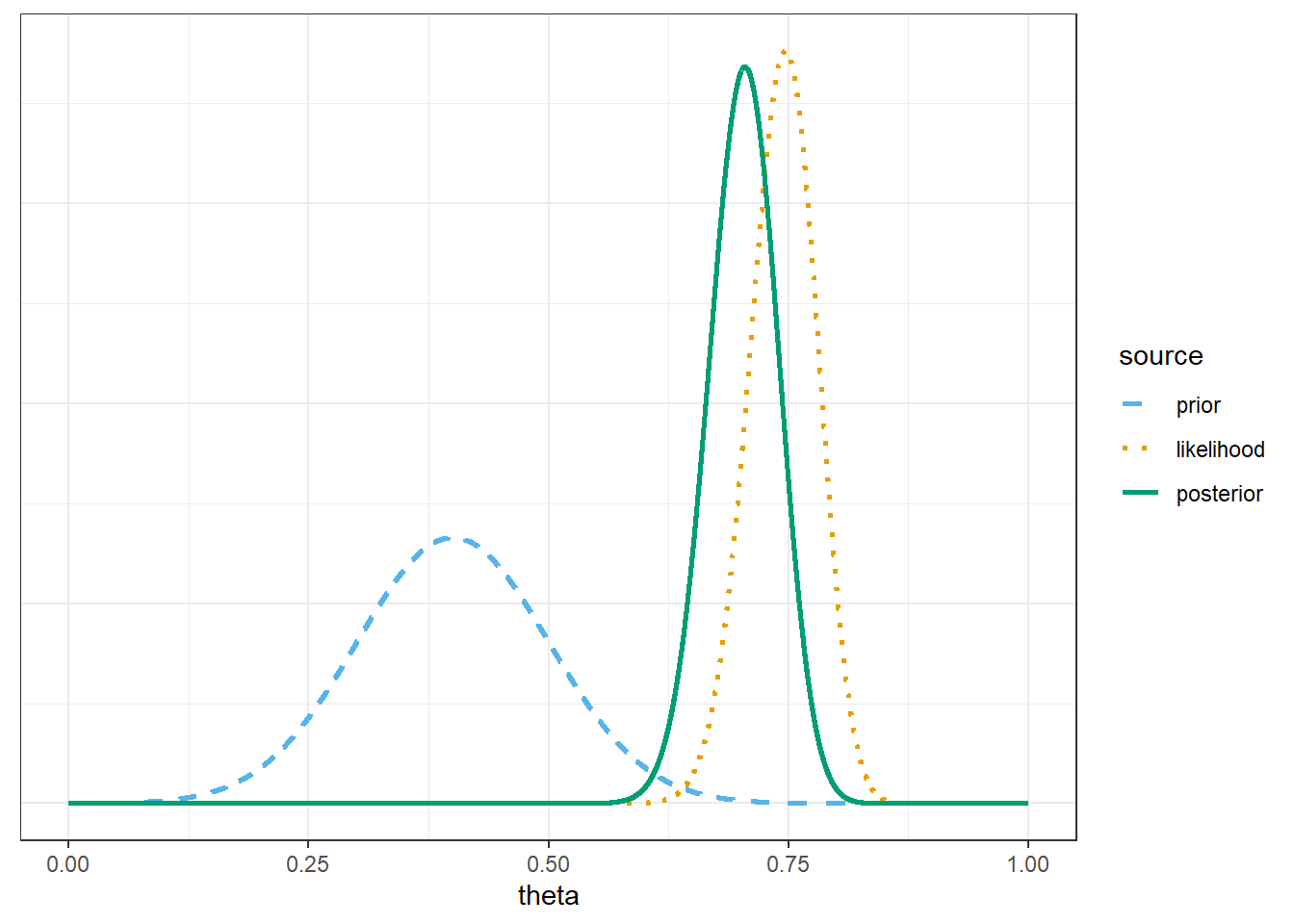
Use grid approximation to approximate the posterior distribution. Make a plot of prior, likelihood, and posterior. Describe the shape of the posterior distribution, and approximate the posterior mean and posterior SD.
The posterior distribution is approximately Normal with posterior mean 0.709 and posterior SD 0.036. How does the sample mean compare, roughly, to the prior mean and the observed sample proportion?
How does the posterior standard deviation compare to the prior standard deviation? Why?
Compute and interpret the posterior probability that \(\theta\) is greater than 0.7. Compare to the prior probability.
Find the 25th and 75th percentiles of the posterior distribution. What is the posterior probability that \(\theta\) lies in the interval with these percentiles as endpoints? According to the posterior, how plausible is it for \(\theta\) to lie inside this interval relative to outside it? Compare to the prior interval.
Repeat the previous part with the 10th and 90th percentiles of the posterior distribution.
Repeat the previous part with the 1st and 99th percentiles of the posterior distribution.

Bayesian inference for a parameter is based on its posterior distribution.
Since a Bayesian analysis treats parameters as random variables, it is possible to make probability statements about a parameter.
A Bayesian credible interval is an interval of values for the parameter that has at least the specified probability, e.g., 50%, 80%, 98%.
- With a 50% credible interval, it is equally plausible that the parameter lies inside the interval as outside
- With an 80% credible interval, it is 4 times more plausible that the parameter lies inside the interval than outside
- With a 98% credible interval, it is 49 times more plausible that the parameter lies inside the interval than outside
Central credible intervals split the complementary probability evenly between the two tails.
- The endpoints of a 50% central posterior credible interval are the 25th and the 75th percentiles of the posterior distribution.
- The endpoints of an 80% central posterior credible interval are the 10th and the 90th percentiles of the posterior distribution.
- The endpoints of a 98% central posterior credible interval are the 1st and the 99th percentiles of the posterior distribution.
Bayesian inference is based on the full posterior distribution. Credible intervals simply provide a summary of this distribution.
Reporting a few credible intervals, rather than just one, provides a richer picture of how the posterior distribution represents the uncertainty in the parameter.
In many situations, the posterior distribution of a single parameter is approximately Normal, so posterior probabilities can be approximated with Normal distribution calculations. If the posterior distribution of a parameter is approximately Normal, an approximate central credible interval has endpoints \[ \text{posterior mean} \pm z^* \times \text{posterior SD} \] where the multiple (a.k.a., critical value) which corresponds to the credibility level comes from a Normal distribution, e.g.,

Central credibility	50%	80%	95%	98%
Normal \(z^*\) multiple	0.67	1.28	1.96	2.33

Example 7.4 Continuing Example 7.1, we’ll assume a Normal prior distribution for \(\theta\) with prior mean 0.4 and prior standard deviation 0.1.

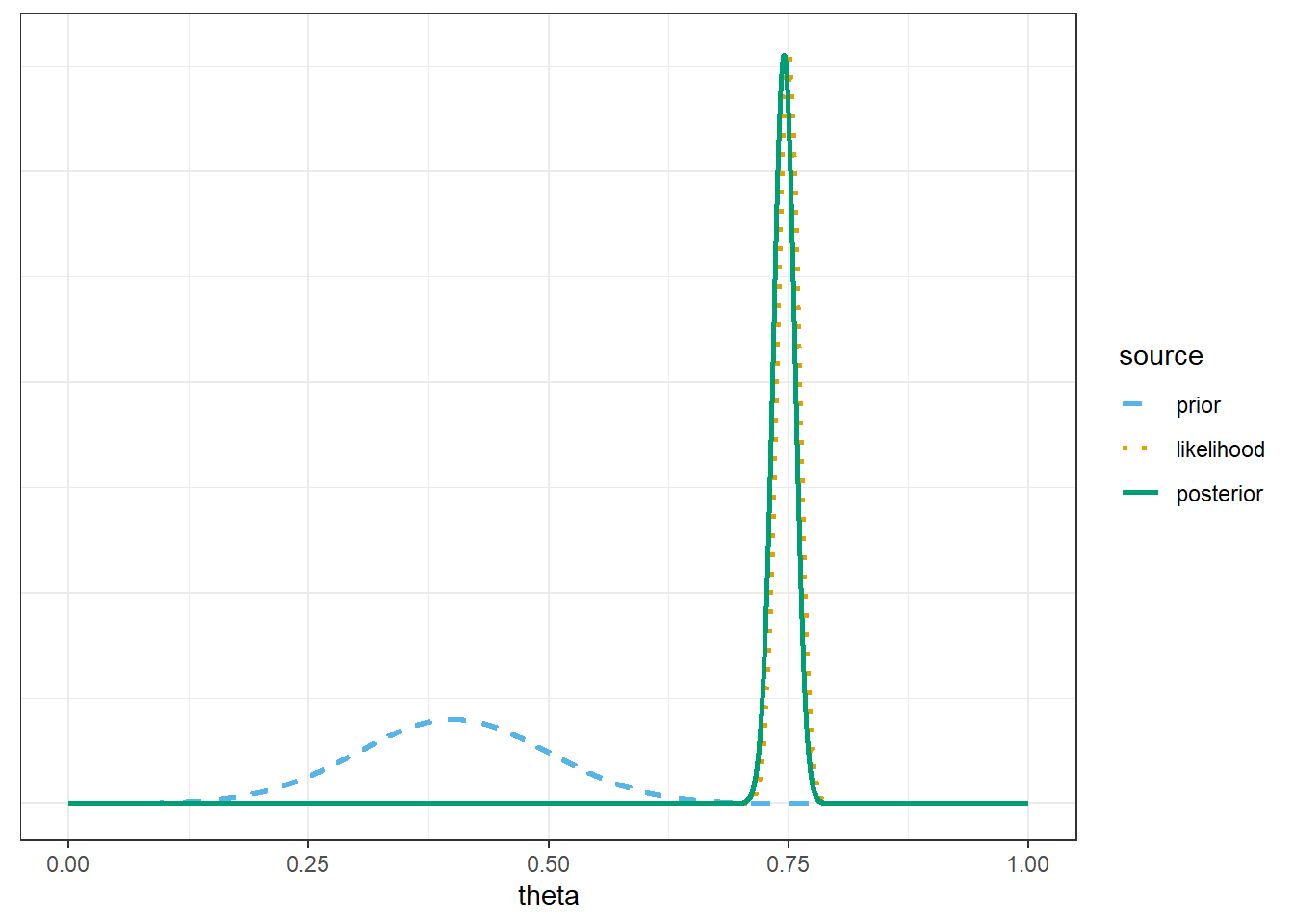
In a recent survey of 1502 American adults conducted by the Pew Research Center, 75% of those surveyed said they have read a book in the past year.

Use grid approximation to approximate the posterior distribution. Make a plot of prior, likelihood, and posterior. Describe the shape of the posterior distribution, and approximate the posterior mean and posterior SD. How does this posterior compare to the one based on the smaller sample size (\(n=150\))?
The posterior distribution is approximately Normal with posterior mean 0.745 and posterior SD 0.011. Compute and interpret in context the posterior probability that \(\theta\) is greater than 0.7. Compare to the prior probability, and to the posterior probability based on the smaller sample size (\(n=150\)).
Compute and interpret in context 50%, 80%, and 98% central posterior credible intervals for \(\theta\). Compare to the prior intervals, and to the posterior intervals based on the smaller sample size (\(n=150\)).
Here is how the survey question was worded: “During the past 12 months, about how many BOOKS did you read either all or part of the way through? Please include any print, electronic, or audiobooks you may have read or listened to.” Does this change your conclusions? Explain.

The quality of any statistical analysis depends very heavily on the quality of the data.
Always investigate how the data were collected to determine what conclusions are appropriate.
Is the sample reasonably representative of the population? Were the variables reliably measured?

Example 7.5 Continuing Example 7.4, we’ll use the same sample data (\(n=1502\), 75%) but now we’ll consider different priors.

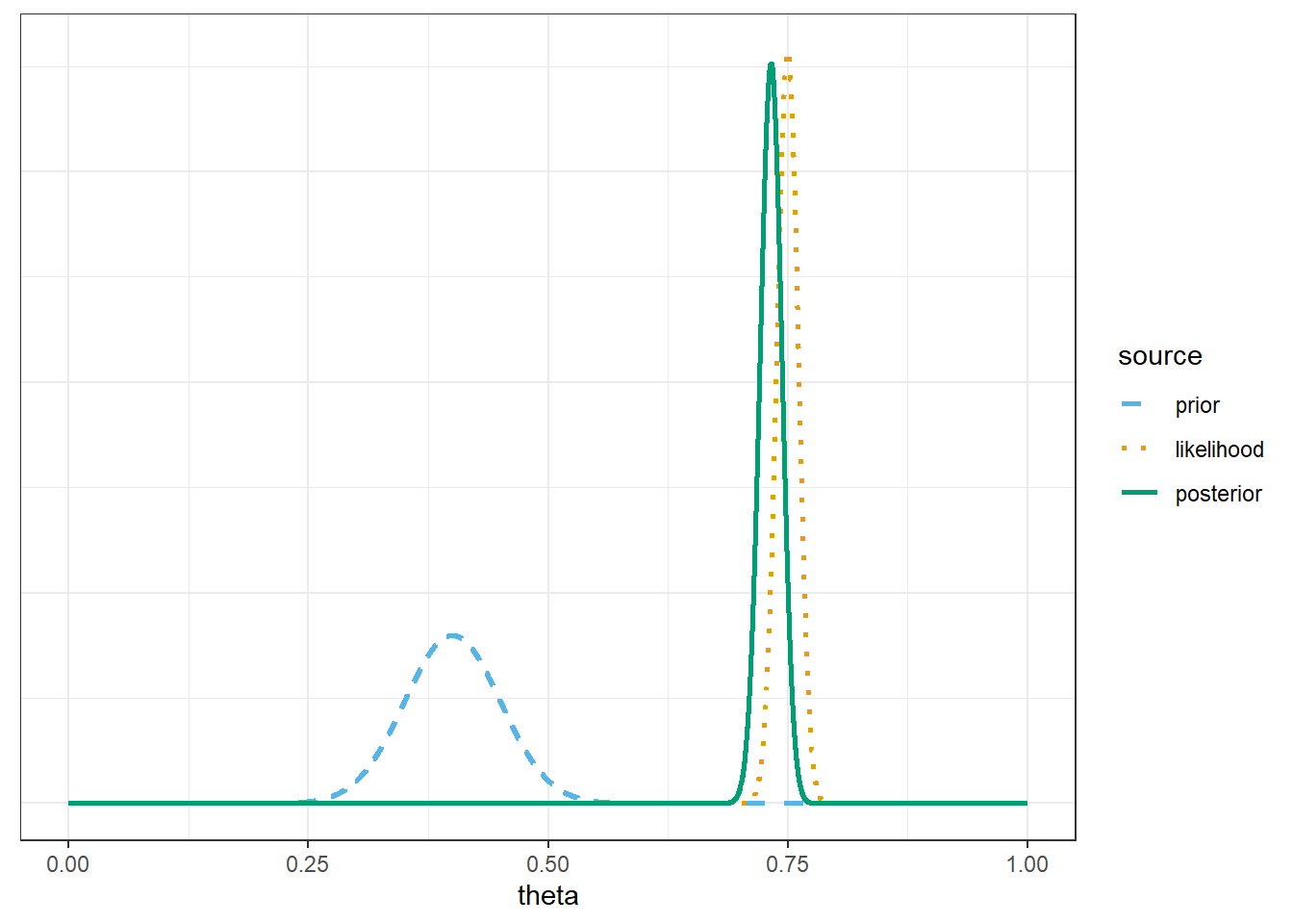
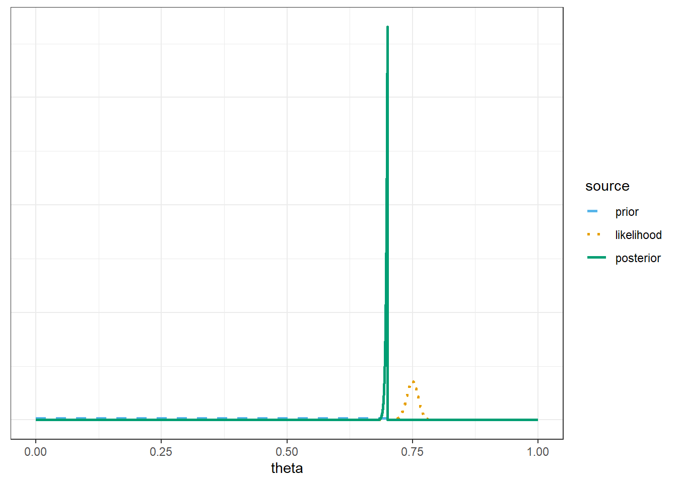
For each of the priors below, plot prior, likelihood, and posterior, and compute the posterior probability that \(\theta\) is greater than 0.7. Compare.

Normal distribution prior with prior mean 0.4 and prior SD 0.05.
Uniform distribution prior on the interval [0, 0.7]

You have a great deal of flexibility in choosing a prior, and there are many reasonable approaches.
However, do NOT choose a prior that assigns 0 probability/density to possible values of the parameter regardless of how initially implausible the values are.

7.1 Notes

7.1.1 Normal(0.4, 0.1) prior

# prior probability theta is greater than 0.7
1 - pnorm(0.7, 0.4, 0.1)

[1] 0.001349898

# endpoints of prior 50% credible interval
qnorm(c(0.25, 0.75), 0.4, 0.1)

[1] 0.332551 0.467449

# endpoints of prior 80% credible interval
qnorm(c(0.10, 0.90), 0.4, 0.1)

[1] 0.2718448 0.5281552

# endpoints of prior 98% credible interval
qnorm(c(0.01, 0.99), 0.4, 0.1)

[1] 0.1673652 0.6326348

7.1.2 Posterior based on sample of size \(n=150\) with \(\hat{p} = 0.75\)

# possible values of theta
theta = seq(0, 1, by = 0.0001)

# prior distribution
prior = dnorm(theta, 0.4, 0.1)
prior = prior / sum(prior)

# observed data
n = 150
y_obs = round(0.75 * n, 0) # sample count of successes

# likelihood of observed data for each theta
likelihood = dbinom(y_obs, n, theta)

# posterior is proportional to product of prior and likelihood
product = prior * likelihood
posterior = product / sum(product)

bayes_table = data.frame(theta,
                         prior,
                         likelihood,
                         product,
                         posterior)

# select a few rows and display them
bayes_table |>
  slice(seq(1001, 9001, 1000)) |> 
  kbl(digits = 8) |>
  kable_styling()

theta	prior	likelihood	product	posterior
0.1	0.00000443	0.00000000	0.0e+00	0.00000000
0.2	0.00005399	0.00000000	0.0e+00	0.00000000
0.3	0.00024198	0.00000000	0.0e+00	0.00000000
0.4	0.00039895	0.00000000	0.0e+00	0.00000000
0.5	0.00024198	0.00000000	0.0e+00	0.00000000
0.6	0.00005399	0.00005945	0.0e+00	0.00002375
0.7	0.00000443	0.03345819	1.5e-07	0.00109713
0.8	0.00000013	0.02128789	0.0e+00	0.00002108
0.9	0.00000000	0.00000004	0.0e+00	0.00000000

bayes_table |>
  # scale likelihood for plotting only
  mutate(likelihood = likelihood / sum(likelihood)) |> 
  select(theta, prior, likelihood, posterior) |>
  pivot_longer(!theta,
               names_to = "source",
               values_to = "probability") |>
  mutate(source = fct_relevel(source, "prior", "likelihood", "posterior")) |>
  ggplot(aes(x = theta,
             y = probability,
             col = source)) +
  geom_line(aes(linetype = source), linewidth = 1) +
  scale_color_manual(values = bayes_col) +
  scale_linetype_manual(values = bayes_lty) +
  theme_bw() +
  # remove y-axis labels
  theme(axis.title.y = element_blank(),
        axis.text.y = element_blank(),
        axis.ticks.y = element_blank())

# posterior mean
post_mean = sum(theta * posterior)
post_mean

[1] 0.7024312

# posterior SD
post_var = sum(theta ^ 2 * posterior) - post_mean ^ 2

post_sd = sqrt(post_var)
post_sd

[1] 0.03597042

# posterior probability theta is greater than 0.7
1 - pnorm(0.7, post_mean, post_sd)

[1] 0.5269438

# endpoints of posterior 50% credible interval
qnorm(c(0.25, 0.75), post_mean, post_sd)

[1] 0.6781695 0.7266929

# endpoints of posterior 80% credible interval
qnorm(c(0.10, 0.90), post_mean, post_sd)

[1] 0.6563333 0.7485292

# endpoints of posterior 98% credible interval
qnorm(c(0.01, 0.99), post_mean, post_sd)

[1] 0.6187515 0.7861109

7.1.3 Posterior based on sample of size \(n=1502\) with \(\hat{p} = 0.75\)

Only change is the sample data.

# possible values of theta
theta = seq(0, 1, by = 0.0001)

# prior distribution
prior = dnorm(theta, 0.4, 0.1)
prior = prior / sum(prior)

# observed data
n = 1502
y_obs = round(0.75 * n, 0) # sample count of successes

# likelihood of observed data for each theta
likelihood = dbinom(y_obs, n, theta)

# posterior is proportional to product of prior and likelihood
product = prior * likelihood
posterior = product / sum(product)

bayes_table = data.frame(theta,
                         prior,
                         likelihood,
                         product,
                         posterior)

# select a few rows and display them
bayes_table |>
  slice(seq(1001, 9001, 1000)) |> 
  kbl(digits = 8) |>
  kable_styling()

theta	prior	likelihood	posterior
0.1	0.00000443	0.00e+00	0.00e+00
0.2	0.00005399	0.00e+00	0.00e+00
0.3	0.00024198	0.00e+00	0.00e+00
0.4	0.00039895	0.00e+00	0.00e+00
0.5	0.00024198	0.00e+00	0.00e+00
0.6	0.00005399	0.00e+00	0.00e+00
0.7	0.00000443	2.57e-06	1.78e-06
0.8	0.00000013	3.10e-07	1.00e-08
0.9	0.00000000	0.00e+00	0.00e+00

bayes_table |>
  # scale likelihood for plotting only
  mutate(likelihood = likelihood / sum(likelihood)) |> 
  select(theta, prior, likelihood, posterior) |>
  pivot_longer(!theta,
               names_to = "source",
               values_to = "probability") |>
  mutate(source = fct_relevel(source, "prior", "likelihood", "posterior")) |>
  ggplot(aes(x = theta,
             y = probability,
             col = source)) +
  geom_line(aes(linetype = source), linewidth = 1) +
  scale_color_manual(values = bayes_col) +
  scale_linetype_manual(values = bayes_lty) +
  theme_bw() +
  # remove y-axis labels
  theme(axis.title.y = element_blank(),
        axis.text.y = element_blank(),
        axis.ticks.y = element_blank())

# posterior mean
post_mean = sum(theta * posterior)
post_mean

[1] 0.7449843

# posterior SD
post_var = sum(theta ^ 2 * posterior) - post_mean ^ 2

post_sd = sqrt(post_var)
post_sd

[1] 0.01122754

# posterior probability theta is greater than 0.7
1 - pnorm(0.7, post_mean, post_sd)

[1] 0.9999692

# endpoints of posterior 50% credible interval
qnorm(c(0.25, 0.75), post_mean, post_sd)

[1] 0.7374115 0.7525572

# endpoints of posterior 80% credible interval
qnorm(c(0.10, 0.90), post_mean, post_sd)

[1] 0.7305956 0.7593730

# endpoints of posterior 98% credible interval
qnorm(c(0.01, 0.99), post_mean, post_sd)

[1] 0.7188652 0.7711035

7.1.4 Conclusions

The posterior probability that \(\theta\) is greater than 0.7 is about 0.9999. We started with only a 0.1% chance that more than 70% of American adults have read a book in the last year, but the large sample has convinced us otherwise.
There is a posterior probability of:
- 50% that the population proportion of American adults who have read a book in the past year is between 0.737 and 0.753. We believe that the population proportion is as likely to be inside this interval as outside.
- 80% that the population proportion of American adults who have read a book in the past year is between 0.730 and 0.759. We believe that the population proportion is four times more likely to be inside this interval than to be outside it.
- 98% that the population proportion of American adults who have read a book in the past year is between 0.718 and 0.771. We believe that the population proportion is 49 times more likely to be inside this interval than to be outside it.
In short, our conclusion is that somewhere-in-the-70s percent of American adults have read a book in the past year (but be careful about what qualifies as “reading a book”.)

7.1.5 Posterior based on Normal(0.4, 0.05) prior

Only change is the prior

# possible values of theta
theta = seq(0, 1, by = 0.0001)

# prior distribution
prior = dnorm(theta, 0.4, 0.05)
prior = prior / sum(prior)

# observed data
n = 1502
y_obs = round(0.75 * n, 0) # sample count of successes

# likelihood of observed data for each theta
likelihood = dbinom(y_obs, n, theta)

# posterior is proportional to product of prior and likelihood
product = prior * likelihood
posterior = product / sum(product)

bayes_table = data.frame(theta,
                         prior,
                         likelihood,
                         product,
                         posterior)

bayes_table |>
  # scale likelihood for plotting only
  mutate(likelihood = likelihood / sum(likelihood)) |> 
  select(theta, prior, likelihood, posterior) |>
  pivot_longer(!theta,
               names_to = "source",
               values_to = "probability") |>
  mutate(source = fct_relevel(source, "prior", "likelihood", "posterior")) |>
  ggplot(aes(x = theta,
             y = probability,
             col = source)) +
  geom_line(aes(linetype = source), linewidth = 1) +
  scale_color_manual(values = bayes_col) +
  scale_linetype_manual(values = bayes_lty) +
  theme_bw() +
  # remove y-axis labels
  theme(axis.title.y = element_blank(),
        axis.text.y = element_blank(),
        axis.ticks.y = element_blank())

# posterior mean
post_mean = sum(theta * posterior)
post_mean

[1] 0.73204

# posterior SD
post_var = sum(theta ^ 2 * posterior) - post_mean ^ 2

post_sd = sqrt(post_var)
post_sd

[1] 0.01135316

# posterior probability theta is greater than 0.7
1 - pnorm(0.7, post_mean, post_sd)

[1] 0.9976147

# endpoints of posterior 50% credible interval
qnorm(c(0.25, 0.75), post_mean, post_sd)

[1] 0.7243824 0.7396976

# endpoints of posterior 80% credible interval
qnorm(c(0.10, 0.90), post_mean, post_sd)

[1] 0.7174903 0.7465897

# endpoints of posterior 98% credible interval
qnorm(c(0.01, 0.99), post_mean, post_sd)

[1] 0.7056286 0.7584514

7.1.6 Posterior based on Uniform(0, 0.7) prior

Only change is the prior

# possible values of theta
theta = seq(0, 1, by = 0.0001)

# prior distribution
prior = dunif(theta, 0, 0.7)
prior = prior / sum(prior)

# observed data
n = 1502
y_obs = round(0.75 * n, 0) # sample count of successes

# likelihood of observed data for each theta
likelihood = dbinom(y_obs, n, theta)

# posterior is proportional to product of prior and likelihood
product = prior * likelihood
posterior = product / sum(product)

bayes_table = data.frame(theta,
                         prior,
                         likelihood,
                         product,
                         posterior)

bayes_table |>
  # scale likelihood for plotting only
  mutate(likelihood = likelihood / sum(likelihood)) |> 
  select(theta, prior, likelihood, posterior) |>
  pivot_longer(!theta,
               names_to = "source",
               values_to = "probability") |>
  mutate(source = fct_relevel(source, "prior", "likelihood", "posterior")) |>
  ggplot(aes(x = theta,
             y = probability,
             col = source)) +
  geom_line(aes(linetype = source), linewidth = 1) +
  scale_color_manual(values = bayes_col) +
  scale_linetype_manual(values = bayes_lty) +
  theme_bw() +
  # remove y-axis labels
  theme(axis.title.y = element_blank(),
        axis.text.y = element_blank(),
        axis.ticks.y = element_blank())

# posterior probability theta is greater than 0.7
sum(posterior[theta > 0.7])

[1] 0