26 Naive Bayes Classification

We have seen how to fit Bayesian regression models for predicting numerical variables. Now we will introduce a Bayesian classification method for predicting categorical variables. The goal is to “classify” observations according to which category (class) they belong to.

This handout corresponds to Chapter 14 of (Johnson, Ott, and Dogucu 2022).

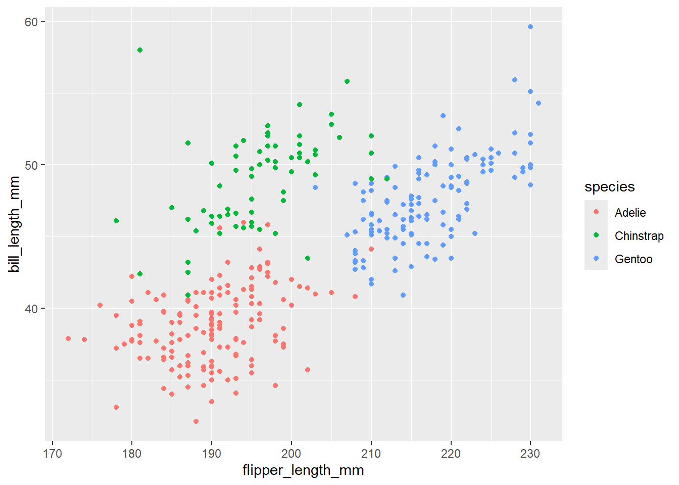
There exist multiple penguin species throughout Antarctica, including the Adelie (A), Chinstrap (C), and Gentoo (G). Our goal will be to classify penguins according to their species given characteristics like weight or bill length. (Throughout “penguin” refers to an Antarctic penguin of one of these three species.)

Example 26.1 Suppose first that we have no information about a randomly selected penguin (other than it’s an Antarctic penguin from one of these three species).

How might we formulate a prior distribution for the species of the penguin? Would we necessarily assume equal prior probability for the three species?
Suppose that among Antarctic penguins of these three species, 44.2% of Adelie, 19.8% are Chinstrap, and 36.0% are Gentoo. Start to set up a Bayes table.

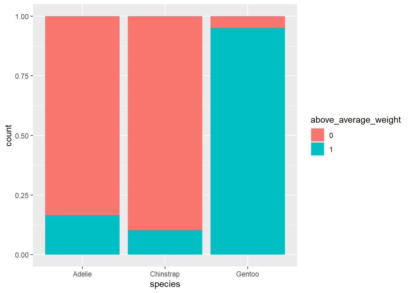
Example 26.2 Now suppose we know that a randomly selected penguin is below average weight (that is, below 4200g).

What is the next column of the Bayes table to fill in? What information would we need to do so?
Suppose that 83.4% of Adelie penguins are below average weight, 89.7% of Chinstrap penguins are below average weight, and 4.9% of Gentoo penguins are below average weight. Among these three species, the likelihood of being below average weight is greatest for Chinstrap. Does that mean we should necessarily classify the penguin to be Chinstrap? Why?
Complete the Bayes table and find the posterior probability of each species given that the penguin is below average weight.
If the species is below average weight, what species would you classify it as? Why?
Now suppose the the species is not below average weight. Compute the posterior probability of each species given that the penguin is not below average weight. What species would you classify it as? Why?
Suppose that you classify any randomly selected penguin based on whether or not it is below average weight. What is the posterior probability that you classify the penguin correctly?

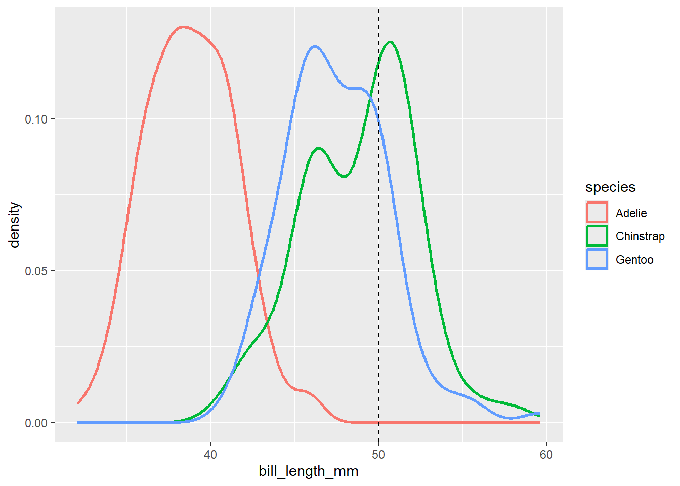
Example 26.3 Now suppose we know that a randomly selected penguin has a bill length of 50mm. We’ll start by assuming we don’t know yet whether or not it is below average weight.

Start to create a Bayes table. What is the prior? What is the next column of the Bayes table to fill in? What information would we need to do so?
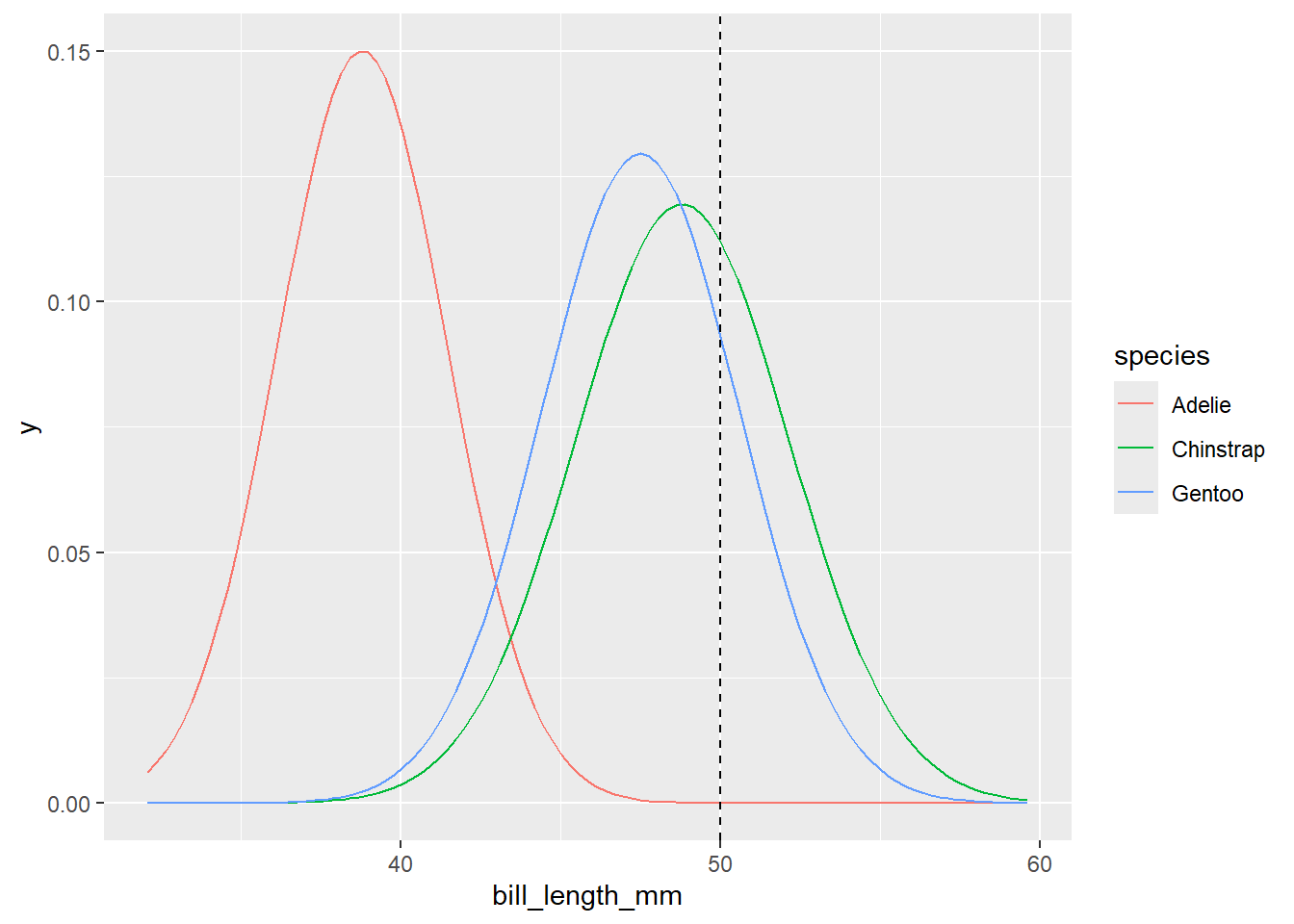
Suppose that bill lengths (mm) follow a N(38.8, 2.66) distribution for Adelie, a N(48.8, 3.34) distribution for Chinstrap, and a N(47.5, 3.08) distribution for Gentoo. How would you fill in the likelihood column?
Among these three species, the likelihood of having of a 50mm bill is greatest for Chinstrap. Does that mean we should necessarily classify the penguin to be Chinstrap? Why?
Complete the Bayes table and find the posterior probability of each species given that the penguin has a 50mm bill.
If the species has a 50mm bill, what species would you classify it as? Why?
Now suppose before measuring bill length we had already known that the penguin was below average weight. How would our Bayes table have changed? If we don’t change the likelihood column, what are we assuming?
Compute the posterior probability of each species given that the penguin is below average weight with a 50mm bill, assuming conditional independence between weight and bill length. Given a species with these characteristics, what species would you classify it as? Why?

Naive Bayes classification uses Bayes rule to predict the class of a categorical response variable \(y\) given predictor variables \(x_1, \ldots, x_p\)
Predictor variables can be categorical or numerical
Naive Bayes classification assumes that predictors are conditionally independent given each class
Naive Bayes classification typically assumes that any numerical predictor variable is conditionally Normal
Given observed data
- Prior probabilities for the response variable are estimated to be the observed sample proportion for each class
- For a categorical predictor \(x\), the likelihood of value \(\tilde{x}\) is estimated to be the observed sample proportion of \(\tilde{x}\) within each class
- For a numerical predictor \(x\), the likelihood is computed assuming that within each class values of the predictor follow a Normal distribution with mean and SD estimated to be the sample mean and SD within each class.

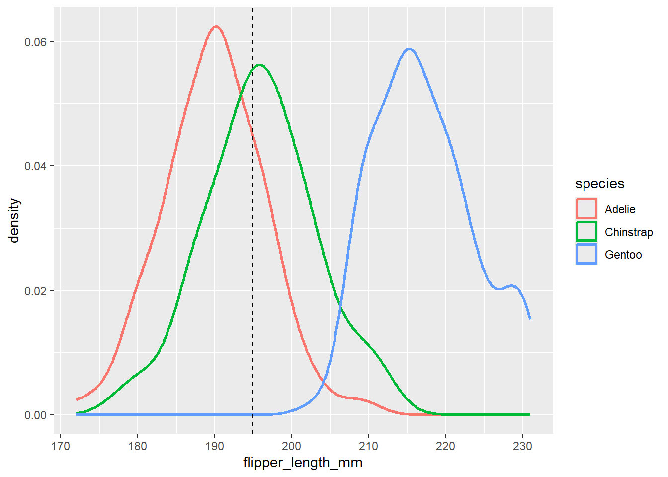
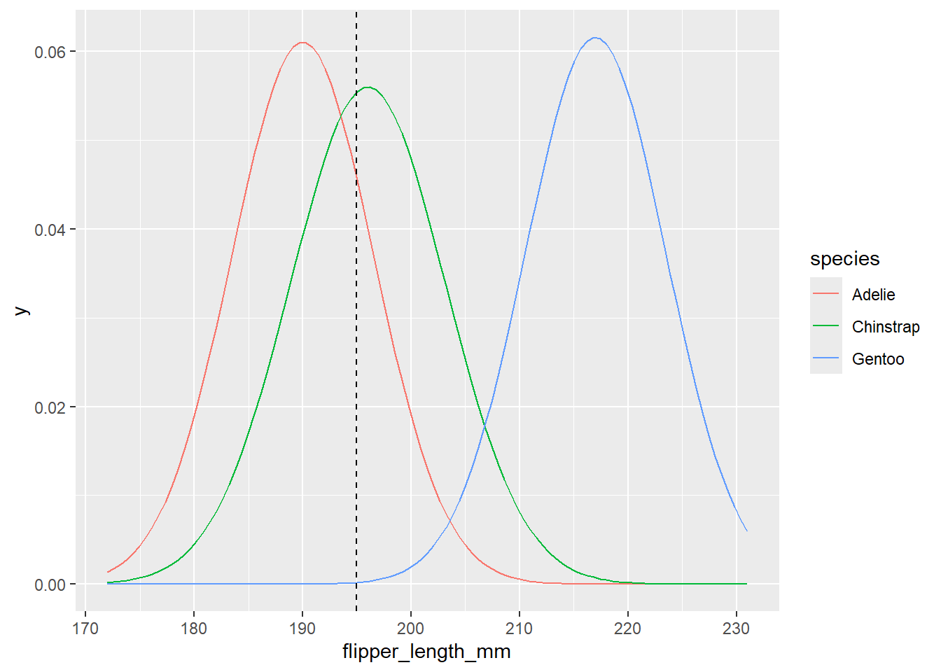
Example 26.4 Now suppose we know that a penguin has a bill length of 50mm and a flipper length of 195mm. (We’ll ignore whether or not it is below average weight for this example.)

Starting with our original prior, what is the “evidence” that the likelihood is based on? What information do we need to fill in the likelihood column?
Suppose that flipper lengths (mm) follow a N(190, 6.54) distribution for Adelie, a N(196, 7.13) distribution for Chinstrap, and a N(217, 6.48) distribution for Gentoo. (Recall that bill lengths (mm) follow a N(38.8, 2.66) distribution for Adelie, a N(48.8, 3.34) distribution for Chinstrap, and a N(47.5, 3.08) distribution for Gentoo.) How would you fill in the likelihood column? What are we assuming?
Complete the Bayes table and find the posterior probability of each species given that the penguin has a 50mm bill and a 195mm flipper.
If the species has a 50mm bill and a 195mm flipper, what species would you classify it as? Why?

26.1 Notes

26.1.1 Given below average weight

class = c("A", "C", "G")

prior = c(0.442, 0.198, 0.360)

# likelihood of below average weight (evidence) given each species (class)
likelihood = c(0.834, 0.897, 0.049) 

product = prior * likelihood

posterior = product / sum(product)

posterior_given_below_average_weight = posterior

bayes_table = data.frame(class,
                         prior,
                         likelihood,
                         product,
                         posterior)

bayes_table |>
  adorn_totals("row") |>
  kbl(digits = 4) |>
  kable_styling()

class	prior	likelihood	product	posterior
A	0.442	0.834	0.3686	0.6537
C	0.198	0.897	0.1776	0.3150
G	0.360	0.049	0.0176	0.0313
Total	1.000	1.780	0.5639	1.0000

26.1.2 Given not below average weight

class = c("A", "C", "G")

prior = c(0.442, 0.198, 0.360)

# likelihood of not below average weight (evidence) given each species (class)
likelihood = c(1 - 0.834, 1 - 0.897, 1 - 0.049) 

product = prior * likelihood

posterior = product / sum(product)

bayes_table = data.frame(class,
                         prior,
                         likelihood,
                         product,
                         posterior)

bayes_table |>
  adorn_totals("row") |>
  kbl(digits = 4) |>
  kable_styling()

class	prior	likelihood	product	posterior
A	0.442	0.166	0.0734	0.1682
C	0.198	0.103	0.0204	0.0468
G	0.360	0.951	0.3424	0.7850
Total	1.000	1.220	0.4361	1.0000

26.1.3 Given 50mm bill

class = c("A", "C", "G")

prior = c(0.442, 0.198, 0.360)

# likelihood of 50mm bill (evidence) given each species (class)
likelihood = c(dnorm(50, 38.8, 2.66),
               dnorm(50, 48.8, 3.34),
               dnorm(50, 47.5, 3.08))

product = prior * likelihood

posterior = product / sum(product)

bayes_table = data.frame(class,
                         prior,
                         likelihood,
                         product,
                         posterior)

bayes_table |>
  adorn_totals("row") |>
  kbl(digits = 4) |>
  kable_styling()

class	prior	likelihood	product	posterior
A	0.442	0.0000	0.0000	0.0002
C	0.198	0.1120	0.0222	0.3979
G	0.360	0.0932	0.0335	0.6019
Total	1.000	0.2052	0.0557	1.0000

26.1.4 Given 50mm bill and below average weight

class = c("A", "C", "G")

prior = posterior_given_below_average_weight

# likelihood of 50mm (evidence) given each species (class)
likelihood = c(dnorm(50, 38.8, 2.66),
               dnorm(50, 48.8, 3.34),
               dnorm(50, 47.5, 3.08))

product = prior * likelihood

posterior = product / sum(product)

bayes_table = data.frame(class,
                         prior,
                         likelihood,
                         product,
                         posterior)

bayes_table |>
  adorn_totals("row") |>
  kbl(digits = 4) |>
  kable_styling()

class	prior	likelihood	product	posterior
A	0.6537	0.0000	0.0000	0.0004
C	0.3150	0.1120	0.0353	0.9233
G	0.0313	0.0932	0.0029	0.0763
Total	1.0000	0.2052	0.0382	1.0000

26.1.5 Given 50mm bill and 195mm flipper

class = c("A", "C", "G")

prior = c(0.442, 0.198, 0.360)

# likelihood of 50mm bill (evidence) given each species (class)
likelihood_bill = c(dnorm(50, 38.8, 2.66),
                    dnorm(50, 48.8, 3.34),
                    dnorm(50, 47.5, 3.08))

# likelihood of 195mm flipper (evidence) given each species (class)
likelihood_flipper = c(dnorm(195, 190, 6.54),
                       dnorm(195, 196, 7.13),
                       dnorm(195, 217, 6.48))

# assume conditional independence of bill and flipper given species (class)
likelihood = likelihood_bill * likelihood_flipper

product = prior * likelihood

posterior = product / sum(product)

bayes_table = data.frame(class,
                         prior,
                         likelihood_bill,
                         likelihood_flipper,
                         likelihood,
                         product,
                         posterior)

bayes_table |>
  adorn_totals("row") |>
  kbl(digits = 6) |>
  kable_styling()

class	prior	likelihood_bill	likelihood_flipper	likelihood	product	posterior
A	0.442	0.000021	0.045542	0.000001	0.000000	0.000345
C	0.198	0.111978	0.055405	0.006204	0.001228	0.994404
G	0.360	0.093174	0.000193	0.000018	0.000006	0.005251
Total	1.000	0.205173	0.101140	0.006223	0.001235	1.000000

26.1.6 Data

This code is taken from Chapter 14 of (Johnson, Ott, and Dogucu 2022).

library(bayesrules)


# Load data
data(penguins_bayes)
penguins <- penguins_bayes

head(penguins)

# A tibble: 6 × 9
  species island     year bill_length_mm bill_depth_mm flipper_length_mm
  <fct>   <fct>     <int>          <dbl>         <dbl>             <int>
1 Adelie  Torgersen  2007           39.1          18.7               181
2 Adelie  Torgersen  2007           39.5          17.4               186
3 Adelie  Torgersen  2007           40.3          18                 195
4 Adelie  Torgersen  2007           NA            NA                  NA
5 Adelie  Torgersen  2007           36.7          19.3               193
6 Adelie  Torgersen  2007           39.3          20.6               190
# ℹ 3 more variables: body_mass_g <int>, above_average_weight <fct>, sex <fct>

Estimated prior distribution

penguins |>
  tabyl(species)

   species   n   percent
    Adelie 152 0.4418605
 Chinstrap  68 0.1976744
    Gentoo 124 0.3604651

Estimated likelihood of below average weight

penguins |>
  select(species, above_average_weight) |>
  na.omit() |>
  tabyl(species, above_average_weight) |>
  adorn_totals(c("row", "col"))

   species   0   1 Total
    Adelie 126  25   151
 Chinstrap  61   7    68
    Gentoo   6 117   123
     Total 193 149   342

ggplot(penguins |>
         drop_na(above_average_weight), 
       aes(fill = above_average_weight,
           x = species)) + 
  geom_bar(position = "fill")

Estimated likelihood of 50mm bill

ggplot(penguins,
       aes(x = bill_length_mm,
           col = species)) + 
  geom_density(linewidth = 1) + 
  geom_vline(xintercept = 50, linetype = "dashed")

Warning: Removed 2 rows containing non-finite outside the scale range
(`stat_density()`).

penguins |>
  group_by(species) |>
  summarize(mean = mean(bill_length_mm, na.rm = TRUE), 
            sd = sd(bill_length_mm, na.rm = TRUE))

# A tibble: 3 × 3
  species    mean    sd
  <fct>     <dbl> <dbl>
1 Adelie     38.8  2.66
2 Chinstrap  48.8  3.34
3 Gentoo     47.5  3.08

ggplot(penguins, aes(x = bill_length_mm, color = species)) + 
  stat_function(fun = dnorm, args = list(mean = 38.8, sd = 2.66), 
                aes(color = "Adelie")) +
  stat_function(fun = dnorm, args = list(mean = 48.8, sd = 3.34),
                aes(color = "Chinstrap")) +
  stat_function(fun = dnorm, args = list(mean = 47.5, sd = 3.08),
                aes(color = "Gentoo")) + 
  geom_vline(xintercept = 50, linetype = "dashed")

Estimated likelihood of 195mm bill

ggplot(penguins,
       aes(x = flipper_length_mm,
           col = species)) + 
  geom_density(linewidth = 1) + 
  geom_vline(xintercept = 195, linetype = "dashed")

Warning: Removed 2 rows containing non-finite outside the scale range
(`stat_density()`).

penguins |>
  group_by(species) |>
  summarize(mean = mean(flipper_length_mm, na.rm = TRUE), 
            sd = sd(flipper_length_mm, na.rm = TRUE))

# A tibble: 3 × 3
  species    mean    sd
  <fct>     <dbl> <dbl>
1 Adelie     190.  6.54
2 Chinstrap  196.  7.13
3 Gentoo     217.  6.48

ggplot(penguins,
       aes(x = flipper_length_mm,
           color = species)) + 
  stat_function(fun = dnorm, args = list(mean = 190, sd = 6.54), 
                aes(color = "Adelie")) +
  stat_function(fun = dnorm, args = list(mean = 196, sd = 7.13),
                aes(color = "Chinstrap")) +
  stat_function(fun = dnorm, args = list(mean = 217, sd = 6.48),
                aes(color = "Gentoo")) + 
  geom_vline(xintercept = 195, linetype = "dashed")

Flipper length and bill length

ggplot(penguins,
       aes(x = flipper_length_mm,
           y = bill_length_mm,
           color = species)) + 
  geom_point()

Warning: Removed 2 rows containing missing values or values outside the scale range
(`geom_point()`).

26.1.7 Naive Bayes Classification with `e1071` package

library(e1071)

our_penguin <- data.frame(above_average_weight = "0",
                          bill_length_mm = 50,
                          flipper_length_mm = 195)

26.1.7.1 Given below average weight

naive_model_weight = naiveBayes(species ~ above_average_weight,
                                data = penguins)

naive_model_weight


Naive Bayes Classifier for Discrete Predictors

Call:
naiveBayes.default(x = X, y = Y, laplace = laplace)

A-priori probabilities:
Y
   Adelie Chinstrap    Gentoo 
0.4418605 0.1976744 0.3604651 

Conditional probabilities:
           above_average_weight
Y                    0          1
  Adelie    0.83443709 0.16556291
  Chinstrap 0.89705882 0.10294118
  Gentoo    0.04878049 0.95121951

predict(naive_model_weight,
        newdata = our_penguin,
        type = "raw")

        Adelie Chinstrap     Gentoo
[1,] 0.6541796 0.3146224 0.03119806

26.1.7.2 Given 50mm bill

naive_model_bill = naiveBayes(species ~ bill_length_mm,
                                data = penguins)

naive_model_bill


Naive Bayes Classifier for Discrete Predictors

Call:
naiveBayes.default(x = X, y = Y, laplace = laplace)

A-priori probabilities:
Y
   Adelie Chinstrap    Gentoo 
0.4418605 0.1976744 0.3604651 

Conditional probabilities:
           bill_length_mm
Y               [,1]     [,2]
  Adelie    38.79139 2.663405
  Chinstrap 48.83382 3.339256
  Gentoo    47.50488 3.081857

predict(naive_model_bill,
        newdata = our_penguin,
        type = "raw")

           Adelie Chinstrap    Gentoo
[1,] 0.0001690279 0.3978306 0.6020004

26.1.7.3 Given 50mm bill and below average weight

naive_model_weight_and_bill = naiveBayes(species ~ above_average_weight + bill_length_mm,
                                         data = penguins)

naive_model_weight_and_bill


Naive Bayes Classifier for Discrete Predictors

Call:
naiveBayes.default(x = X, y = Y, laplace = laplace)

A-priori probabilities:
Y
   Adelie Chinstrap    Gentoo 
0.4418605 0.1976744 0.3604651 

Conditional probabilities:
           above_average_weight
Y                    0          1
  Adelie    0.83443709 0.16556291
  Chinstrap 0.89705882 0.10294118
  Gentoo    0.04878049 0.95121951

           bill_length_mm
Y               [,1]     [,2]
  Adelie    38.79139 2.663405
  Chinstrap 48.83382 3.339256
  Gentoo    47.50488 3.081857

predict(naive_model_weight_and_bill,
        newdata = our_penguin,
        type = "raw")

           Adelie Chinstrap     Gentoo
[1,] 0.0003650334 0.9236333 0.07600171

26.1.7.4 Given 50mm bill and 195mm flipper

naive_model_flipper_and_bill = naiveBayes(species ~ flipper_length_mm + bill_length_mm,
                                          data = penguins)

naive_model_flipper_and_bill


Naive Bayes Classifier for Discrete Predictors

Call:
naiveBayes.default(x = X, y = Y, laplace = laplace)

A-priori probabilities:
Y
   Adelie Chinstrap    Gentoo 
0.4418605 0.1976744 0.3604651 

Conditional probabilities:
           flipper_length_mm
Y               [,1]     [,2]
  Adelie    189.9536 6.539457
  Chinstrap 195.8235 7.131894
  Gentoo    217.1870 6.484976

           bill_length_mm
Y               [,1]     [,2]
  Adelie    38.79139 2.663405
  Chinstrap 48.83382 3.339256
  Gentoo    47.50488 3.081857

predict(naive_model_flipper_and_bill,
        newdata = our_penguin,
        type = "raw")

           Adelie Chinstrap      Gentoo
[1,] 0.0003445688 0.9948681 0.004787365

26.1.7.5 Evaluation of flipper length and bill length model

Can classify each of the penguins in the data set

penguins <- penguins %>%
  mutate(predicted_species = predict(naive_model_flipper_and_bill, newdata = .))

penguins |> 
  select(bill_length_mm, flipper_length_mm, species, predicted_species) |>
  head(10) |>
  kbl() |> kable_styling()

bill_length_mm	flipper_length_mm	species	predicted_species
39.1	181	Adelie	Adelie
39.5	186	Adelie	Adelie
40.3	195	Adelie	Adelie
NA	NA	Adelie	Adelie
36.7	193	Adelie	Adelie
39.3	190	Adelie	Adelie
38.9	181	Adelie	Adelie
39.2	195	Adelie	Adelie
34.1	193	Adelie	Adelie
42.0	190	Adelie	Adelie

Then check classification against actual species to see how well the classification algorithm works within the sample.

penguins |>
  tabyl(species, predicted_species) |>
  adorn_percentages("row") |>
  adorn_pct_formatting(digits = 2) |>
  adorn_ns()

   species       Adelie   Chinstrap       Gentoo
    Adelie 96.05% (146)  2.63%  (4)  1.32%   (2)
 Chinstrap  7.35%   (5) 86.76% (59)  5.88%   (4)
    Gentoo  0.81%   (1)  0.81%  (1) 98.39% (122)

We can use cross-validation to estimate how well our algorithm would classify new penguins outside of the data set.

naive_cv <-
  naive_classification_summary_cv(model = naive_model_flipper_and_bill,
                                  data = penguins,
                                  y = "species",
                                  k = 10)

naive_cv$cv

   species       Adelie   Chinstrap       Gentoo
    Adelie 96.05% (146)  2.63%  (4)  1.32%   (2)
 Chinstrap  7.35%   (5) 86.76% (59)  5.88%   (4)
    Gentoo  0.81%   (1)  0.81%  (1) 98.39% (122)