dbinom(8, size = 12, prob = 0.1)[1] 3.247695e-06Example 6.1 Most people are right-handed, and even the right eye is dominant for most people. In a 2003 study reported in Nature, a German bio-psychologist conjectured that this preference for the right side manifests itself in other ways as well. In particular, he investigated if people have a tendency to lean their heads to the right when kissing. The researcher observed kissing couples in public places and recorded whether the couple leaned their heads to the right or left. (We’ll assume this represents a randomly selected representative sample of kissing couples.)
The parameter of interest is the population proportion of kissing couples who lean their heads to the right. Denote this unknown parameter \(\theta\); our goal is to estimate \(\theta\) based on sample data. We’ll take a Bayesian approach to estimating \(\theta\): we’ll treat the unknown parameter \(\theta\) as a random variable and wish to find its posterior distribution after observing data on a sample of \(n\) kissing couples of which \(y\) lean their heads to the right.
Sketch a distribution representing your plausibility assessment of \(\theta\) prior to observing the sample data.
We will start with a very simplified, unrealistic prior distribution that assumes only five possible, equally likely values for \(\theta\): 0.1, 0.3, 0.5, 0.7, 0.9. Sketch the prior distribution and start constructing a Bayes table.
Now suppose that we observe a sample of \(n=12\) kissing couples of which \(y=8\) lean right. Describe in principle would you fill in the likelihood column.
If \(\theta=0.1\) what is the distribution of \(y\)? Compute and interpret the probability that \(y=8\) if \(\theta = 0.1\).
If \(\theta=0.3\) what is the distribution of \(y\)? Compute and interpret the probability that \(y=8\) if \(\theta = 0.3\).
If \(\theta=0.5\) what is the distribution of \(y\)? Compute and interpret the probability that \(y=8\) if \(\theta = 0.5\).
If \(\theta=0.7\) what is the distribution of \(y\)? Compute and interpret the probability that \(y=8\) if \(\theta = 0.7\).
If \(\theta=0.9\) what is the distribution of \(y\)? Compute and interpret the probability that \(y=8\) if \(\theta = 0.9\).
Sketch a plot of the likelihood function and fill in the likelihood column in the Bayes table.
Complete the Bayes table and sketch a plot of the posterior distribution.
Examine the posterior distribution. What does it say about \(\theta\)? How does it compare to the prior and the likelihood?
Now consider a prior distribution which places probability 1/9, 2/9, 3/9, 2/9, 1/9 on the values 0.1, 0.3, 0.5, 0.7, 0.9, respectively. Assuming the same sample data (\(y/n = 8/12\)), construct a Bayes table using this prior. How does the posterior distribution compare to the one based on the equally likely prior?
Now consider a prior distribution which places probability 5/15, 4/15, 3/15, 2/15, 1/15 on the values 0.1, 0.3, 0.5, 0.7, 0.9, respectively. Assuming the same sample data (\(y/n = 8/12\)), construct a Bayes table using this prior. How does the posterior distribution compare to the ones from the previous parts?
Example 6.2 Continuing Example 6.1. While the previous exercise introduced the main ideas, it was unrealistic to consider only five possible values of \(\theta\).
What are the possible values of \(\theta\)? Does the parameter \(\theta\) take values on a continuous or discrete scale? (Careful: we’re talking about the parameter and not the data.)
Let’s assume that any multiple of 0.0001 is a possible value of \(\theta\): \(0, 0.0001, 0.0002, \ldots, 0.9999, 1\). Assume a discrete uniform (equally likely) prior distribution on these values. Suppose again that \(y=8\) couples in a sample of \(n=12\) kissing couples lean right. Use software to plot the prior distribution, the (scaled) likelihood function, and then find the posterior and plot it. Describe the posterior distribution. What does it say about \(\theta\)?
Now assume a prior distribution which is proportional to \(1-2|\theta-0.5|\) for \(\theta = 0, 0.0001, 0.0002, \ldots, 0.9999, 1\). Use software to plot this prior; what does it say about \(\theta\)? Then suppose again that \(y=8\) couples in a sample of \(n=12\) kissing couples lean right. Use software to plot the prior distribution, the (scaled) likelihood function, and then find the posterior and plot it. What does the posterior distribution say about \(\theta\)?
Now assume a prior distribution which is proportional to \(1-\theta\) for \(\theta = 0, 0.0001, 0.0002, \ldots, 0.9999, 1\). Use software to plot this prior; what does it say about \(\theta\)? Then suppose again that \(y=8\) couples in a sample of \(n=12\) kissing couples lean right. Use software to plot the prior distribution, the (scaled) likelihood function, and then find the posterior and plot it. What does the posterior distribution say about \(\theta\)?
Compare the posterior distributions corresponding to the three different priors. How does each posterior distribution compare to the prior and the likelihood? Does the prior distribution influence the posterior distribution?
Example 6.3 Continuing Example 6.2. Now we’ll perform a Bayesian analysis on the actual study data in which \(y=80\) couples out of a sample of \(n=124\) leaned right. We’ll again use a grid approximation and assume that any multiple of 0.0001 between 0 and 1 is a possible value of \(\theta\): \(0, 0.0001, 0.0002, \ldots, 0.9999, 1\).
Before performing the Bayesian analysis, use software to plot the likelihood when \(y=80\) couples in a sample of \(n=124\) kissing couples lean right. How does the likelihood for this sample compare to the likelihood based on the smaller sample (8/12) from previous exercises?
Now back to Bayesian analysis. Assume a discrete uniform prior distribution for \(\theta\). Suppose that \(y=80\) couples in a sample of \(n=124\) kissing couples lean right. Use software to plot the prior distribution, the likelihood function, and then find the posterior and plot it. Describe the posterior distribution. What does it say about \(\theta\)?
Now assume a prior distribution which is proportional to \(1-2|\theta-0.5|\) for \(\theta = 0, 0.0001, 0.0002, \ldots, 0.9999, 1\). Then suppose again that \(y=80\) couples in a sample of \(n=124\) kissing couples lean right. Use software to plot the prior distribution, the likelihood function, and then find the posterior and plot it. What does the posterior distribution say about \(\theta\)?
Now assume a prior distribution which is proportional to \(1-\theta\) for \(\theta = 0, 0.0001, 0.0002, \ldots, 0.9999, 1\). Then suppose again that \(y=80\) couples in a sample of \(n=124\) kissing couples lean right. Use software to plot the prior distribution, the likelihood function, and then find the posterior and plot it. What does the posterior distribution say about \(\theta\)?
Compare the posterior distributions corresponding to the three different priors. How does each posterior distribution compare to the prior and the likelihood? Comment on the influence that the prior distribution has. Does the Bayesian inference for this data appear to be highly sensitive to the choice of prior? How does this compare to the \(n=12\) situation?
If you had to produce a single number Bayesian estimate of \(\theta\) based on the sample data, what number might you pick?
Example 6.4 Continuing Example 6.1 where \(\theta\) can only take values 0.1, 0.3, 0.5, 0.7, 0.9. Consider a prior distribution which places probability 5/15, 4/15, 3/15, 2/15, 1/15 on the values 0.1, 0.3, 0.5, 0.7, 0.9, respectively. Ssuppose that \(y=8\) couples in a sample of size \(n=12\) lean right. Recall the Bayes table.
Suppose we want a single number point estimate of \(\theta\) before observing sample data. Find the mode of the prior distribution of \(\theta\), a.k.a., the “prior mode”.
Find the expected value of the prior distribution of \(\theta\), a.k.a., the “prior mean”.
Suppose we want a single number point estimate of \(\theta\) after observing sample data. Find the mode of the posterior distribution of \(\theta\), a.k.a., the “posterior mode”.
Find the expected value of the prior distribution of \(\theta\), a.k.a., the “posterior mean”. How does the posterior mean compare to the prior mean and the observed sample propotion?
If \(\theta=0.1\) the likelihood of \(y=8\) when \(n=12\) is
dbinom(8, size = 12, prob = 0.1)[1] 3.247695e-06If \(\theta=0.3\) the likelihood of \(y=8\) when \(n=12\) is
dbinom(8, 12, 0.3)[1] 0.007797716If \(\theta=0.5\) the likelihood of \(y=8\) when \(n=12\) is
dbinom(8, 12, 0.5)[1] 0.1208496If \(\theta=0.7\) the likelihood of \(y=8\) when \(n=12\) is
dbinom(8, 12, 0.7)[1] 0.2311397If \(\theta=0.9\) the likelihood of \(y=8\) when \(n=12\) is
dbinom(8, 12, 0.9)[1] 0.02130813# possible values of theta
theta = seq(0.1, 0.9, by = 0.2)
# prior distribution
prior = rep(1, length(theta))
prior = prior / sum(prior)
# observed data
n = 12
y_obs = 8
# likelihood of observed data for each theta
likelihood = dbinom(y_obs, n, theta)
# posterior is proportional to product of prior and likelihood
product = prior * likelihood
posterior = product / sum(product)
bayes_table = data.frame(theta,
prior,
likelihood,
product,
posterior)
bayes_table |>
adorn_totals("row") |>
kbl(digits = 4) |>
kable_styling()| theta | prior | likelihood | product | posterior |
|---|---|---|---|---|
| 0.1 | 0.2 | 0.0000 | 0.0000 | 0.0000 |
| 0.3 | 0.2 | 0.0078 | 0.0016 | 0.0205 |
| 0.5 | 0.2 | 0.1208 | 0.0242 | 0.3171 |
| 0.7 | 0.2 | 0.2311 | 0.0462 | 0.6065 |
| 0.9 | 0.2 | 0.0213 | 0.0043 | 0.0559 |
| Total | 1.0 | 0.3811 | 0.0762 | 1.0000 |
bayes_table |>
  # scale likelihood for plotting only
  mutate(likelihood = likelihood / sum(likelihood)) |>
  select(theta, prior, likelihood, posterior) |>
  pivot_longer(!theta,
               names_to = "source",
               values_to = "prob") |>
  mutate(source = fct_relevel(source, "prior", "likelihood", "posterior")) |>
  ggplot(aes(x = theta,
             y = prob,
             col = source)) +
  geom_point(size = 3) +
  geom_line(aes(linetype = source)) +
  scale_x_continuous(breaks = theta) +
  scale_color_manual(values = bayes_col) +
  scale_linetype_manual(values = bayes_lty) +
  labs(y = "Probability") +
  theme_bw()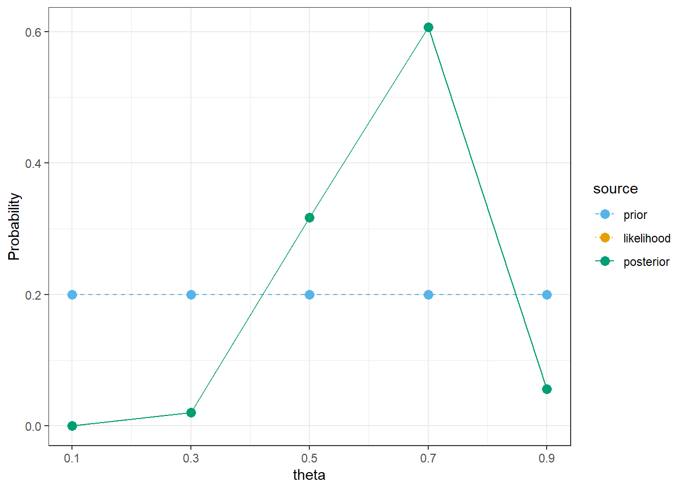
# prior mean
sum(theta * prior)
[1] 0.5# posterior mean
sum(theta * posterior)[1] 0.6395712The only code change is the prior
# possible values of theta
theta = seq(0.1, 0.9, by = 0.2)

# prior distribution
prior = c(1, 2, 3, 2, 1)
prior = prior / sum(prior)

# observed data
n = 12
y_obs = 8

# likelihood of observed data for each theta
likelihood = dbinom(y_obs, n, theta)

# posterior is proportional to product of prior and likelihood
product = prior * likelihood
posterior = product / sum(product)

bayes_table = data.frame(theta,
                         prior,
                         likelihood,
                         product,
                         posterior)

bayes_table |>
  adorn_totals("row") |>
  kbl(digits = 4) |>
kable_styling()| theta | prior | likelihood | product | posterior |
|---|---|---|---|---|
| 0.1 | 0.1111 | 0.0000 | 0.0000 | 0.0000 |
| 0.3 | 0.2222 | 0.0078 | 0.0017 | 0.0181 |
| 0.5 | 0.3333 | 0.1208 | 0.0403 | 0.4207 |
| 0.7 | 0.2222 | 0.2311 | 0.0514 | 0.5365 |
| 0.9 | 0.1111 | 0.0213 | 0.0024 | 0.0247 |
| Total | 1.0000 | 0.3811 | 0.0957 | 1.0000 |
bayes_table |>
  # scale likelihood for plotting only
  mutate(likelihood = likelihood / sum(likelihood)) |>
  select(theta, prior, likelihood, posterior) |>
  pivot_longer(!theta,
               names_to = "source",
               values_to = "prob") |>
  mutate(source = fct_relevel(source, "prior", "likelihood", "posterior")) |>
  ggplot(aes(x = theta,
             y = prob,
             col = source)) +
  geom_point(size = 3) +
  geom_line(aes(linetype = source)) +
  scale_x_continuous(breaks = theta) +
  scale_color_manual(values = bayes_col) +
  scale_linetype_manual(values = bayes_lty) +
  labs(y = "Probability") +
  theme_bw()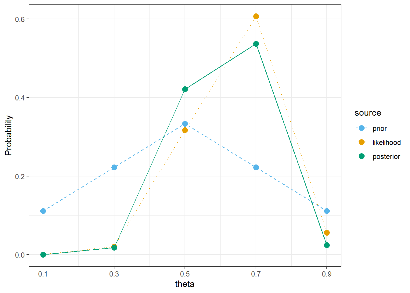
# prior mean
sum(theta * prior)
[1] 0.5# posterior mean
sum(theta * posterior)[1] 0.6135601The only code change is the prior
# possible values of theta
theta = seq(0.1, 0.9, by = 0.2)

# prior distribution
prior = c(5, 4, 3, 2, 1)
prior = prior / sum(prior)

# observed data
n = 12
y_obs = 8

# likelihood of observed data for each theta
likelihood = dbinom(y_obs, n, theta)

# posterior is proportional to product of prior and likelihood
product = prior * likelihood
posterior = product / sum(product)

bayes_table = data.frame(theta,
                         prior,
                         likelihood,
                         product,
                         posterior)

bayes_table |>
  adorn_totals("row") |>
  kbl(digits = 4) |>
kable_styling()| theta | prior | likelihood | product | posterior |
|---|---|---|---|---|
| 0.1 | 0.3333 | 0.0000 | 0.0000 | 0.0000 |
| 0.3 | 0.2667 | 0.0078 | 0.0021 | 0.0356 |
| 0.5 | 0.2000 | 0.1208 | 0.0242 | 0.4132 |
| 0.7 | 0.1333 | 0.2311 | 0.0308 | 0.5269 |
| 0.9 | 0.0667 | 0.0213 | 0.0014 | 0.0243 |
| Total | 1.0000 | 0.3811 | 0.0585 | 1.0000 |
bayes_table |>
  # scale likelihood for plotting only
  mutate(likelihood = likelihood / sum(likelihood)) |>
  select(theta, prior, likelihood, posterior) |>
  pivot_longer(!theta,
               names_to = "source",
               values_to = "prob") |>
  mutate(source = fct_relevel(source, "prior", "likelihood", "posterior")) |>
  ggplot(aes(x = theta,
             y = prob,
             col = source)) +
  geom_point(size = 3) +
  geom_line(aes(linetype = source)) +
  scale_x_continuous(breaks = theta) +
  scale_color_manual(values = bayes_col) +
  scale_linetype_manual(values = bayes_lty) +
  labs(y = "Probability") +
  theme_bw()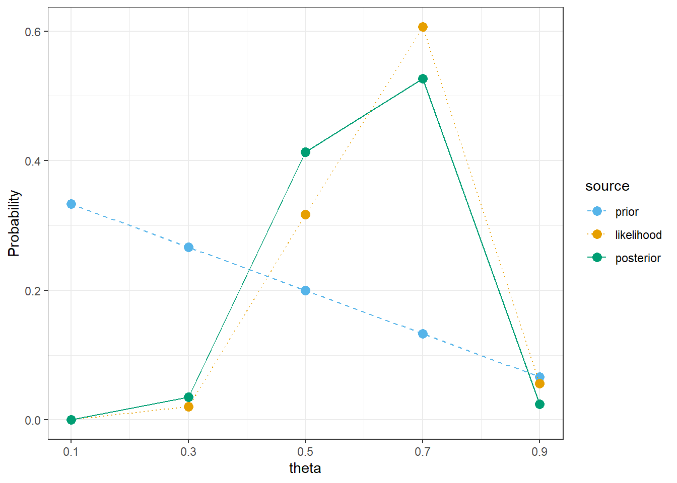
# prior mean
sum(theta * prior)
[1] 0.3666667# posterior mean
sum(theta * posterior)[1] 0.6079788The only real code change is to have a longer grid of theta values. (There are some small changes to the plot, and only selected rows in the Bayes table are displayed.)
# possible values of theta
theta = seq(0, 1, by = 0.0001)

# prior distribution
prior = rep(1, length(theta))
prior = prior / sum(prior)

# observed data
n = 12
y_obs = 8

# likelihood of observed data for each theta
likelihood = dbinom(y_obs, n, theta)

# posterior is proportional to product of prior and likelihood
product = prior * likelihood
posterior = product / sum(product)

bayes_table = data.frame(theta,
                         prior,
                         likelihood,
                         product,
                         posterior)

bayes_table |>
  # select a few rows to display
  slice(seq(5001, 7001, 250)) |>
  kbl(digits = 8) |>
kable_styling()| theta | prior | likelihood | product | posterior |
|---|---|---|---|---|
| 0.500 | 9.999e-05 | 0.1208496 | 1.208e-05 | 0.00015710 |
| 0.525 | 9.999e-05 | 0.1454300 | 1.454e-05 | 0.00018906 |
| 0.550 | 9.999e-05 | 0.1699639 | 1.699e-05 | 0.00022095 |
| 0.575 | 9.999e-05 | 0.1929762 | 1.930e-05 | 0.00025087 |
| 0.600 | 9.999e-05 | 0.2128409 | 2.128e-05 | 0.00027669 |
| 0.625 | 9.999e-05 | 0.2279137 | 2.279e-05 | 0.00029629 |
| 0.650 | 9.999e-05 | 0.2366923 | 2.367e-05 | 0.00030770 |
| 0.675 | 9.999e-05 | 0.2379955 | 2.380e-05 | 0.00030939 |
| 0.700 | 9.999e-05 | 0.2311397 | 2.311e-05 | 0.00030048 |
bayes_table |>
  # scale likelihood for plotting only
  mutate(likelihood = likelihood / sum(likelihood)) |>
  select(theta, prior, likelihood, posterior) |>
  pivot_longer(!theta,
               names_to = "source",
               values_to = "probability") |>
  mutate(source = fct_relevel(source, "prior", "likelihood", "posterior")) |>
  ggplot(aes(x = theta,
             y = probability,
             col = source)) +
  geom_line(aes(linetype = source), linewidth = 1) +
  scale_color_manual(values = bayes_col) +
  scale_linetype_manual(values = bayes_lty) +
  theme_bw()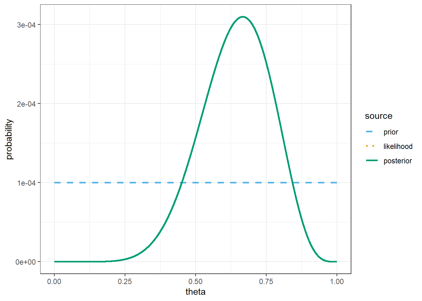
# prior mean
sum(theta * prior)
[1] 0.5# posterior mean
sum(theta * posterior)[1] 0.6428571The only change is the prior.
# possible values of theta
theta = seq(0, 1, by = 0.0001)

# prior distribution
prior = 1 - 2 * abs(theta - 0.5)
prior = prior / sum(prior)

# observed data
n = 12
y_obs = 8

# likelihood of observed data for each theta
likelihood = dbinom(y_obs, n, theta)

# posterior is proportional to product of prior and likelihood
product = prior * likelihood
posterior = product / sum(product)

bayes_table = data.frame(theta,
                         prior,
                         likelihood,
                         product,
                         posterior)

bayes_table |>
  # select a few rows to display
  slice(seq(5001, 7001, 250)) |>
  kbl(digits = 8) |>
kable_styling()| theta | prior | likelihood | product | posterior |
|---|---|---|---|---|
| 0.500 | 0.00020 | 0.1208496 | 2.417e-05 | 0.00023161 |
| 0.525 | 0.00019 | 0.1454300 | 2.763e-05 | 0.00026478 |
| 0.550 | 0.00018 | 0.1699639 | 3.059e-05 | 0.00029317 |
| 0.575 | 0.00017 | 0.1929762 | 3.281e-05 | 0.00031437 |
| 0.600 | 0.00016 | 0.2128409 | 3.405e-05 | 0.00032633 |
| 0.625 | 0.00015 | 0.2279137 | 3.419e-05 | 0.00032760 |
| 0.650 | 0.00014 | 0.2366923 | 3.314e-05 | 0.00031754 |
| 0.675 | 0.00013 | 0.2379955 | 3.094e-05 | 0.00029648 |
| 0.700 | 0.00012 | 0.2311397 | 2.774e-05 | 0.00026579 |
bayes_table |>
  # scale likelihood for plotting only
  mutate(likelihood = likelihood / sum(likelihood)) |>
  select(theta, prior, likelihood, posterior) |>
  pivot_longer(!theta,
               names_to = "source",
               values_to = "probability") |>
  mutate(source = fct_relevel(source, "prior", "likelihood", "posterior")) |>
  ggplot(aes(x = theta,
             y = probability,
             col = source)) +
  geom_line(aes(linetype = source), linewidth = 1) +
  scale_color_manual(values = bayes_col) +
  scale_linetype_manual(values = bayes_lty) +
  theme_bw()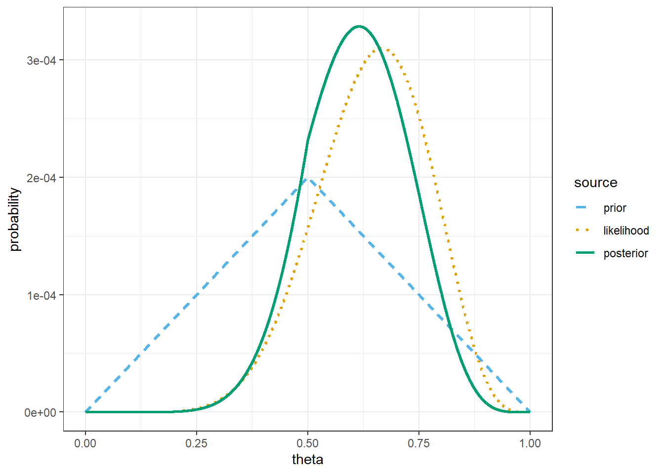
# prior mean
sum(theta * prior)
[1] 0.5# posterior mean
sum(theta * posterior)[1] 0.6113453The only change is the prior.
# possible values of theta
theta = seq(0, 1, by = 0.0001)

# prior distribution
prior = 1 - theta
prior = prior / sum(prior)

# observed data
n = 12
y_obs = 8

# likelihood of observed data for each theta
likelihood = dbinom(y_obs, n, theta)

# posterior is proportional to product of prior and likelihood
product = prior * likelihood
posterior = product / sum(product)

bayes_table = data.frame(theta,
                         prior,
                         likelihood,
                         product,
                         posterior)

bayes_table |>
  # select a few rows to display
  slice(seq(5001, 7001, 250)) |>
  kbl(digits = 8) |>
kable_styling()| theta | prior | likelihood | product | posterior |
|---|---|---|---|---|
| 0.500 | 9.999e-05 | 0.1208496 | 1.208e-05 | 0.00021995 |
| 0.525 | 9.499e-05 | 0.1454300 | 1.381e-05 | 0.00025145 |
| 0.550 | 8.999e-05 | 0.1699639 | 1.530e-05 | 0.00027840 |
| 0.575 | 8.499e-05 | 0.1929762 | 1.640e-05 | 0.00029853 |
| 0.600 | 7.999e-05 | 0.2128409 | 1.703e-05 | 0.00030990 |
| 0.625 | 7.499e-05 | 0.2279137 | 1.709e-05 | 0.00031110 |
| 0.650 | 6.999e-05 | 0.2366923 | 1.657e-05 | 0.00030155 |
| 0.675 | 6.499e-05 | 0.2379955 | 1.547e-05 | 0.00028155 |
| 0.700 | 5.999e-05 | 0.2311397 | 1.387e-05 | 0.00025240 |
bayes_table |>
  # scale likelihood for plotting only
  mutate(likelihood = likelihood / sum(likelihood)) |>
  select(theta, prior, likelihood, posterior) |>
  pivot_longer(!theta,
               names_to = "source",
               values_to = "probability") |>
  mutate(source = fct_relevel(source, "prior", "likelihood", "posterior")) |>
  ggplot(aes(x = theta,
             y = probability,
             col = source)) +
  geom_line(aes(linetype = source), linewidth = 1) +
  scale_color_manual(values = bayes_col) +
  scale_linetype_manual(values = bayes_lty) +
  theme_bw()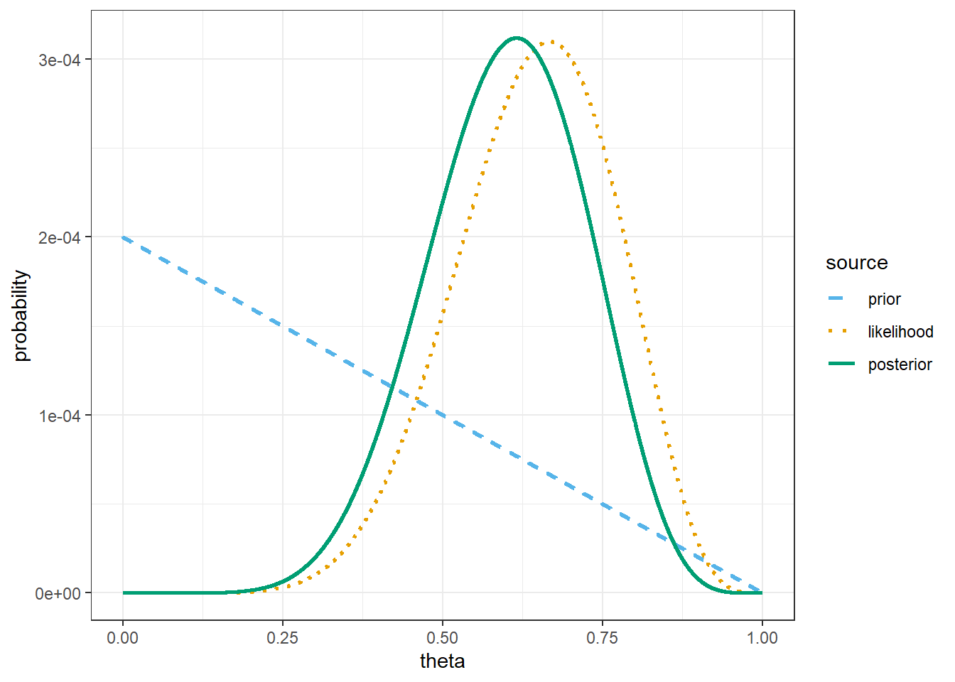
# prior mean
sum(theta * prior)
[1] 0.3333# posterior mean
sum(theta * posterior)[1] 0.6The only code change is to the observed data.
# possible values of theta
theta = seq(0, 1, by = 0.0001)

# prior distribution
prior = rep(1, length(theta))
prior = prior / sum(prior)

# observed data
n = 124
y_obs = 80

# likelihood of observed data for each theta
likelihood = dbinom(y_obs, n, theta)

# posterior is proportional to product of prior and likelihood
product = prior * likelihood
posterior = product / sum(product)

bayes_table = data.frame(theta,
                         prior,
                         likelihood,
                         product,
                         posterior)

bayes_table |>
  # select a few rows to display
  slice(seq(5001, 7001, 250)) |>
  kbl(digits = 8) |>
kable_styling()| theta | prior | likelihood | product | posterior |
|---|---|---|---|---|
| 0.500 | 9.999e-05 | 0.00037224 | 4.00e-08 | 0.00000465 |
| 0.525 | 9.999e-05 | 0.00193109 | 1.90e-07 | 0.00002414 |
| 0.550 | 9.999e-05 | 0.00739443 | 7.40e-07 | 0.00009243 |
| 0.575 | 9.999e-05 | 0.02094495 | 2.09e-06 | 0.00026181 |
| 0.600 | 9.999e-05 | 0.04378027 | 4.38e-06 | 0.00054725 |
| 0.625 | 9.999e-05 | 0.06703721 | 6.70e-06 | 0.00083797 |
| 0.650 | 9.999e-05 | 0.07423373 | 7.42e-06 | 0.00092792 |
| 0.675 | 9.999e-05 | 0.05830536 | 5.83e-06 | 0.00072882 |
| 0.700 | 9.999e-05 | 0.03160219 | 3.16e-06 | 0.00039503 |
bayes_table |>
  # scale likelihood for plotting only
  mutate(likelihood = likelihood / sum(likelihood)) |>
  select(theta, prior, likelihood, posterior) |>
  pivot_longer(!theta,
               names_to = "source",
               values_to = "probability") |>
  mutate(source = fct_relevel(source, "prior", "likelihood", "posterior")) |>
  ggplot(aes(x = theta,
             y = probability,
             col = source)) +
  geom_line(aes(linetype = source), linewidth = 1) +
  scale_color_manual(values = bayes_col) +
  scale_linetype_manual(values = bayes_lty) +
  theme_bw()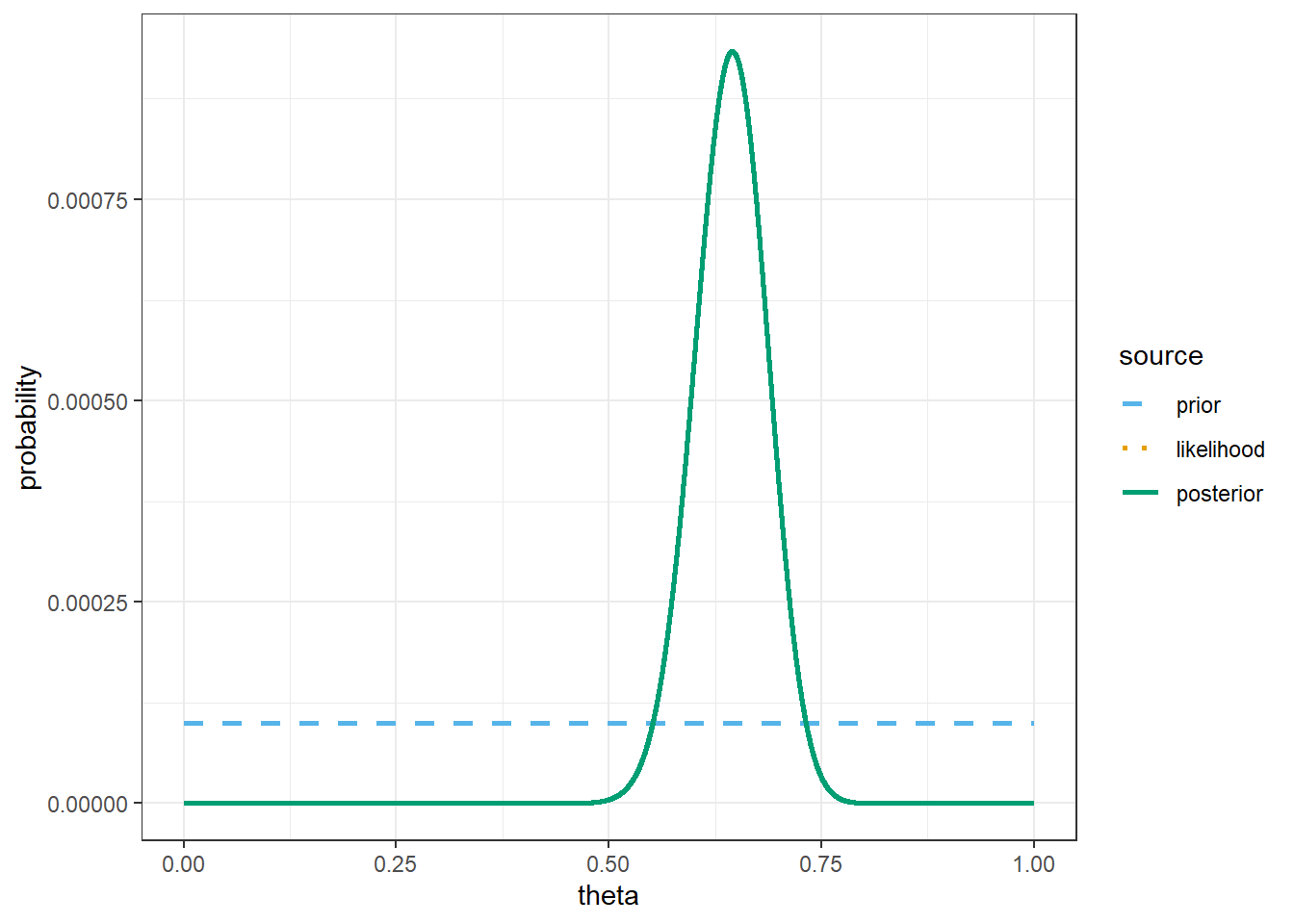
# prior mean
sum(theta * prior)
[1] 0.5# posterior mean
sum(theta * posterior)[1] 0.6428571The only change is the prior.
# possible values of theta
theta = seq(0, 1, by = 0.0001)

# prior distribution
prior = 1 - 2 * abs(theta - 0.5)
prior = prior / sum(prior)

# observed data
n = 124
y_obs = 80

# likelihood of observed data for each theta
likelihood = dbinom(y_obs, n, theta)

# posterior is proportional to product of prior and likelihood
product = prior * likelihood
posterior = product / sum(product)

bayes_table = data.frame(theta,
                         prior,
                         likelihood,
                         product,
                         posterior)

bayes_table |>
  # select a few rows to display
  slice(seq(5001, 7001, 250)) |>
  kbl(digits = 8) |>
kable_styling()| theta | prior | likelihood | product | posterior |
|---|---|---|---|---|
| 0.500 | 0.00020 | 0.00037224 | 7.000e-08 | 0.00000651 |
| 0.525 | 0.00019 | 0.00193109 | 3.700e-07 | 0.00003211 |
| 0.550 | 0.00018 | 0.00739443 | 1.330e-06 | 0.00011647 |
| 0.575 | 0.00017 | 0.02094495 | 3.560e-06 | 0.00031157 |
| 0.600 | 0.00016 | 0.04378027 | 7.000e-06 | 0.00061295 |
| 0.625 | 0.00015 | 0.06703721 | 1.006e-05 | 0.00087990 |
| 0.650 | 0.00014 | 0.07423373 | 1.039e-05 | 0.00090940 |
| 0.675 | 0.00013 | 0.05830536 | 7.580e-06 | 0.00066325 |
| 0.700 | 0.00012 | 0.03160219 | 3.790e-06 | 0.00033184 |
bayes_table |>
  # scale likelihood for plotting only
  mutate(likelihood = likelihood / sum(likelihood)) |>
  select(theta, prior, likelihood, posterior) |>
  pivot_longer(!theta,
               names_to = "source",
               values_to = "probability") |>
  mutate(source = fct_relevel(source, "prior", "likelihood", "posterior")) |>
  ggplot(aes(x = theta,
             y = probability,
             col = source)) +
  geom_line(aes(linetype = source), linewidth = 1) +
  scale_color_manual(values = bayes_col) +
  scale_linetype_manual(values = bayes_lty) +
  theme_bw()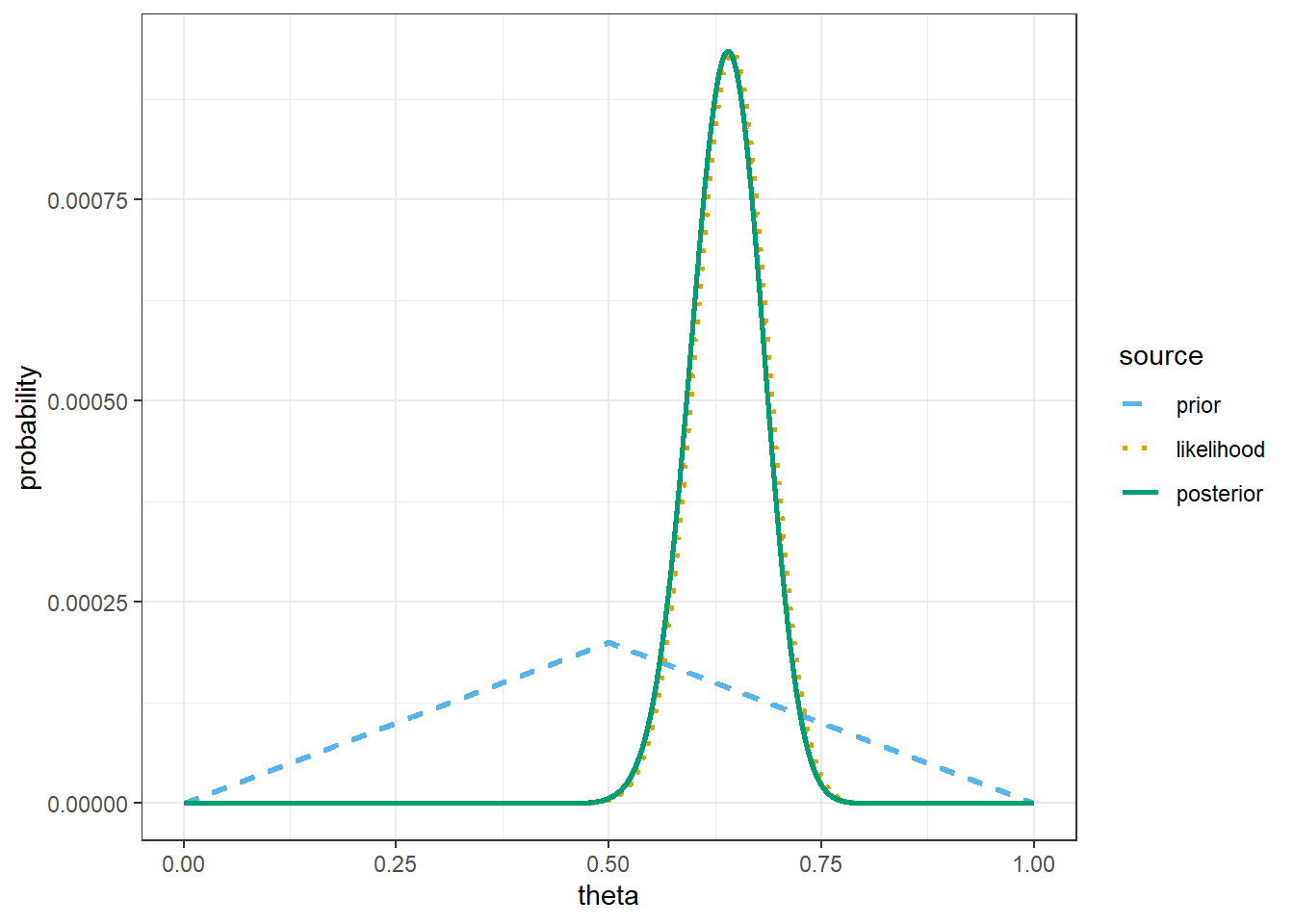
# prior mean
sum(theta * prior)
[1] 0.5# posterior mean
sum(theta * posterior)[1] 0.6378017The only change is the prior.
# possible values of theta
theta = seq(0, 1, by = 0.0001)

# prior distribution
prior = 1 - theta
prior = prior / sum(prior)

# observed data
n = 124
y_obs = 80

# likelihood of observed data for each theta
likelihood = dbinom(y_obs, n, theta)

# posterior is proportional to product of prior and likelihood
product = prior * likelihood
posterior = product / sum(product)

bayes_table = data.frame(theta,
                         prior,
                         likelihood,
                         product,
                         posterior)

bayes_table |>
  # select a few rows to display
  slice(seq(5001, 7001, 250)) |>
  kbl(digits = 8) |>
kable_styling()| theta | prior | likelihood | product | posterior |
|---|---|---|---|---|
| 0.500 | 9.999e-05 | 0.00037224 | 4.00e-08 | 0.00000651 |
| 0.525 | 9.499e-05 | 0.00193109 | 1.80e-07 | 0.00003210 |
| 0.550 | 8.999e-05 | 0.00739443 | 6.70e-07 | 0.00011646 |
| 0.575 | 8.499e-05 | 0.02094495 | 1.78e-06 | 0.00031156 |
| 0.600 | 7.999e-05 | 0.04378027 | 3.50e-06 | 0.00061292 |
| 0.625 | 7.499e-05 | 0.06703721 | 5.03e-06 | 0.00087986 |
| 0.650 | 6.999e-05 | 0.07423373 | 5.20e-06 | 0.00090936 |
| 0.675 | 6.499e-05 | 0.05830536 | 3.79e-06 | 0.00066322 |
| 0.700 | 5.999e-05 | 0.03160219 | 1.90e-06 | 0.00033182 |
bayes_table |>
  # scale likelihood for plotting only
  mutate(likelihood = likelihood / sum(likelihood)) |>
  select(theta, prior, likelihood, posterior) |>
  pivot_longer(!theta,
               names_to = "source",
               values_to = "probability") |>
  mutate(source = fct_relevel(source, "prior", "likelihood", "posterior")) |>
  ggplot(aes(x = theta,
             y = probability,
             col = source)) +
  geom_line(aes(linetype = source), linewidth = 1) +
  scale_color_manual(values = bayes_col) +
  scale_linetype_manual(values = bayes_lty) +
  theme_bw()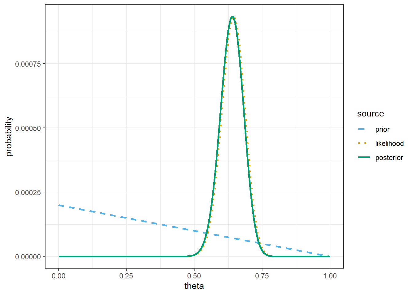
# prior mean
sum(theta * prior)
[1] 0.3333# posterior mean
sum(theta * posterior)[1] 0.6377953# simulate values of theta from the posterior distribution
theta_sim = sample(theta, 10000, replace = TRUE, prob = posterior)
# approximate posterior distribution
hist(theta_sim, freq = FALSE)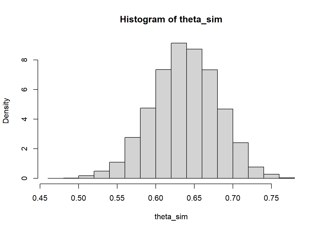
# approximate posterior mean
mean(theta_sim)
[1] 0.6379011# approximate posterior median
median(theta_sim)[1] 0.63835For example, maximum likelihood estimation is a common frequentist technique for estimating the value of a parameter based on data from a sample. The value of a parameter that maximizes the likelihood function is called a maximum likelihood estimate (MLE). The MLE depends on the data \(y\): the MLE is the value of \(\theta\) which gives the largest likelihood of having produced the observed data \(y\).↩︎
In contrast, a frequentist approach regards parameters as unknown but fixed (not random) quantities.↩︎