11 Predictive Tuning and Checking

11.1 Prior predictive tuning

Prior distributions of parameters quantify uncertainty about parameters before observing data.
Considering prior predictive distributions of possible samples under the proposed model can help tune prior distributions of parameters.

Example 11.1 Suppose we’re interested in studying hours of sleep on a typical weeknight for Cal Poly students.

What percent of students do you think sleep more than 10 hours on a typical weeknight? Less than 5 hours?
Suppose we want to perform a Bayesian analysis to estimate \(\theta\), the population mean hours of sleep on a typical weeknight for Cal Poly students. Assume that sleep hours for individual students follow a Normal distribution with unknown mean \(\theta\) and known standard deviation \(\sigma=\) 1.5 hours. (Known population SD is an unrealistic assumption that we use for simplicity here.) Suppose we want to “let the data speak for itself” so we choose a flat, Uniform prior¹. Our Uniform prior needs an upper and lower bound. We remember that we shouldn’t assign 0 prior probability to possible values, no matter how implausible, so we pick a fairly wide range of possible values for \(\theta\), namely Uniform on [3, 13]. Use simulation to approximate the prior predictive distribution of sleep hours according to our model.
According to this model, (approximately) what percent of students sleep more than 10 hours on a typical weeknight? Less than 5? Do these values seem reasonable? If not, what should we do?

Prior predictive distributions “live” on the scale of the data, and are sometimes easier to interpret than prior distributions themselves, especially when there are multiple parameters.
It is often helpful to tune prior distributions of parameters indirectly via prior predictive distributions rather than directly.
We can choose a prior distribution for parameters, simulate a prior predictive distribution for the data (according to our conditional model) given this prior, and consider if the distribution of possible data values seems reasonable given our background knowledge about the variable and context.
If not, we can choose another prior distribution and repeat the process until we have suitably “tuned” the prior distribution for the parameters.
Remember, the prior distribution does not have to be perfect; there is no perfect prior distribution. However, if a particular prior distribution gives rise to obviously unreasonable data values (e.g., negative sleep hours) we should try to improve it. It’s always a good idea to consider prior predictive distributions when formulating a prior distribution for parameters.
Also remember, there are many assumptions that go into any model. If the prior predictive distribution indicates potential inadequacy of the model, it is not necessarily the fault of the prior distribution.

11.2 Posterior predictive checking

Posterior predictive distributions can be used to check if model assumptions seem reasonable in light of observed data.

Example 11.2 Recall Example 10.1 which concerned \(\theta\), the population proportion of students in Cal Poly statistics classes who prefer to consider data as a singular noun (as in “the data is”). Suppose that before collecting data for our sample of Cal Poly students, we had based our prior distribution off the FiveThirtyEight data. In particular, suppose we assume a Normal prior distribution for \(\theta\) with prior mean 0.792 and prior SD 0.012.

What does this our prior distribution say about our beliefs about \(\theta\)?
Now suppose we randomly select a sample of 35 Cal Poly students and 21 students prefer data as singular. Find the posterior distribution, and plot prior, likelihood, and posterior. Have our beliefs about \(\theta\) changed? Why?
Use simulation to find the posterior predictive distribution corresponding to samples of size 35. Compare the observed sample value of 21/35 with the posterior predictive distribution. What do you notice? Does this indicate problems with the model?

A Bayesian model is composed of both a model for the data (likelihood) and a prior distribution on model parameters.
Predictive distributions can be used as tools in model checking.
Posterior predictive checking involves comparing the observed data to simulated samples (or some summary statistics) generated from the posterior predictive distribution.
We’ll focus on graphical checks: Compare plots for the observed data with those for simulated samples. Systematic differences between simulated samples and observed data indicate potential shortcomings of the model.
If the model fits the data, then replicated data generated under the model should look similar to the observed data.
If the observed data is not plausible under the posterior predictive distribution, then this could indicate that the model is not a good fit for the data. (“Based on the data we observed, we conclude that it would be unlikely to observe the data we observed???”)
However, a problematic model isn’t necessarily due to the prior. Remember that a Bayesian model consists of both a prior and a likelihood, so model mis-specification can occur in the prior or likelihood or both. The form of the likelihood is also based on subjective assumptions about the variables being measured and how the data are collected. Posterior predictive checking can help assess whether these assumptions are reasonable in light of the observed data.

Example 11.3 A basketball player will attempt a sequence of 20 free throws. Our model assumes

The probability that the player successfully makes any particular free throw attempt is \(\theta\).
A Uniform prior distribution for \(\theta\) (in a grid from 0 to 1).
Conditional on \(\theta\), the number of successfully made attempts has a Binomial(20, \(\theta\)) distribution. (This determines the likelihood.)

Suppose the player misses her first 10 attempts and makes her second 10 attempts. Does this data seem consistent with the model?
Explain how you could use posterior predictive checking to check the fit of the model.

11.3 Notes

11.3.1 Prior predictive distribution of sleep hours

n_rep = 10000

# simulate theta from prior
theta_sim = runif(n_rep, 3, 13)

# given theta, simulation y from model for data
sigma = 1.5
y_sim = rnorm(n_rep, theta_sim, sigma)

# plot the simulated y values
ggplot(data.frame(y_sim),
       aes(x = y_sim)) + 
  geom_histogram(aes(y = after_stat(density)),
                 col = bayes_col["prior_predict"],
                 fill = "white") +
  geom_density(col = bayes_col["prior_predict"],
               linewidth = 1) +
  labs(x = "Sleep hours (y)") +
  theme_bw()
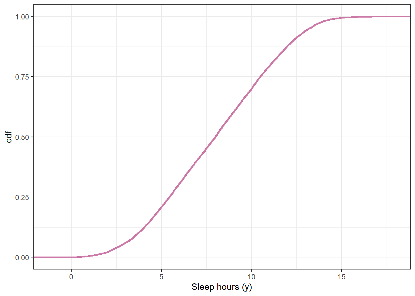
# plot the cdf
ggplot(data.frame(y_sim),
       aes(x = y_sim)) + 
  stat_ecdf(col = bayes_col["prior_predict"],
            linewidth = 1) +
  labs(x = "Sleep hours (y)",
       y = "cdf") +
  theme_bw()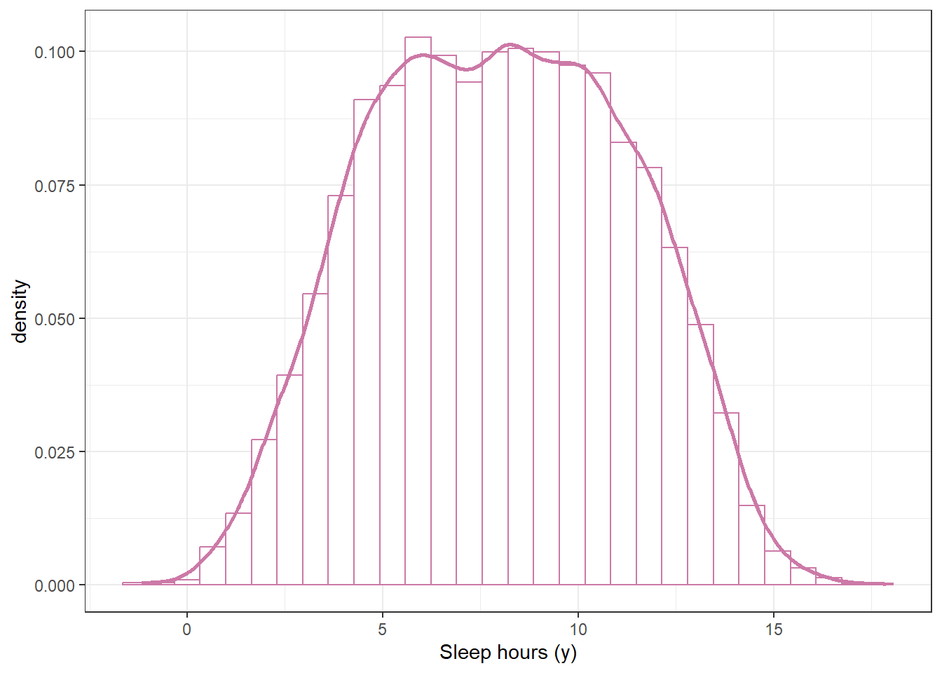

sum(y_sim > 10) / n_rep

[1] 0.3009

sum(y_sim < 5) / n_rep

[1] 0.2086

11.3.2 Posterior predictive checking: Data is singular

# possible values of theta
theta = seq(0, 1, 0.0001)

# prior
prior = dnorm(theta, 0.792, 0.012)
prior = prior / sum(prior)

# observed data
n = 35
y_obs = 21

# likelihood of observed data for each theta
likelihood = dbinom(y_obs, n, theta)

# posterior is proportional to product of prior and likelihood
product = prior * likelihood
posterior = product / sum(product)

bayes_table = data.frame(theta,
                         prior,
                         likelihood,
                         product,
                         posterior)

bayes_table |>
  # scale likelihood for plotting only
  mutate(likelihood = likelihood / sum(likelihood)) |> 
  select(theta, prior, likelihood, posterior) |>
  pivot_longer(!theta,
               names_to = "source",
               values_to = "probability") |>
  mutate(source = fct_relevel(source, "prior", "likelihood", "posterior")) |>
  ggplot(aes(x = theta,
             y = probability,
             col = source)) +
  geom_line(aes(linetype = source), linewidth = 1) +
  scale_color_manual(values = bayes_col) +
  scale_linetype_manual(values = bayes_lty) +
  theme_bw() +
  # remove y-axis labels
  theme(axis.title.y = element_blank(),
        axis.text.y = element_blank(),
        axis.ticks.y = element_blank())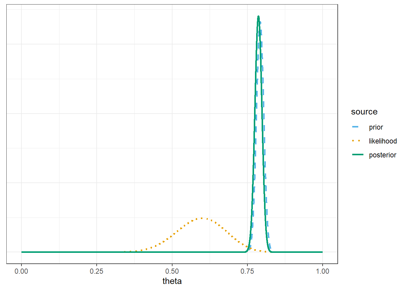

n = 35

n_rep = 10000

# Predictive simulation
theta_sim = sample(theta, n_rep, replace = TRUE, prob = posterior)

y_sim = rbinom(n_rep, n, theta_sim)

ggplot(data.frame(y_sim),
       aes(x = y_sim)) +
  geom_bar(aes(y = after_stat(prop)),
           col = bayes_col["posterior_predict"],
           fill = bayes_col["posterior_predict"],
           width = 0.1) +
  labs(x = "Number of successes",
       y = "Simulated relative frequency") +
  theme_bw()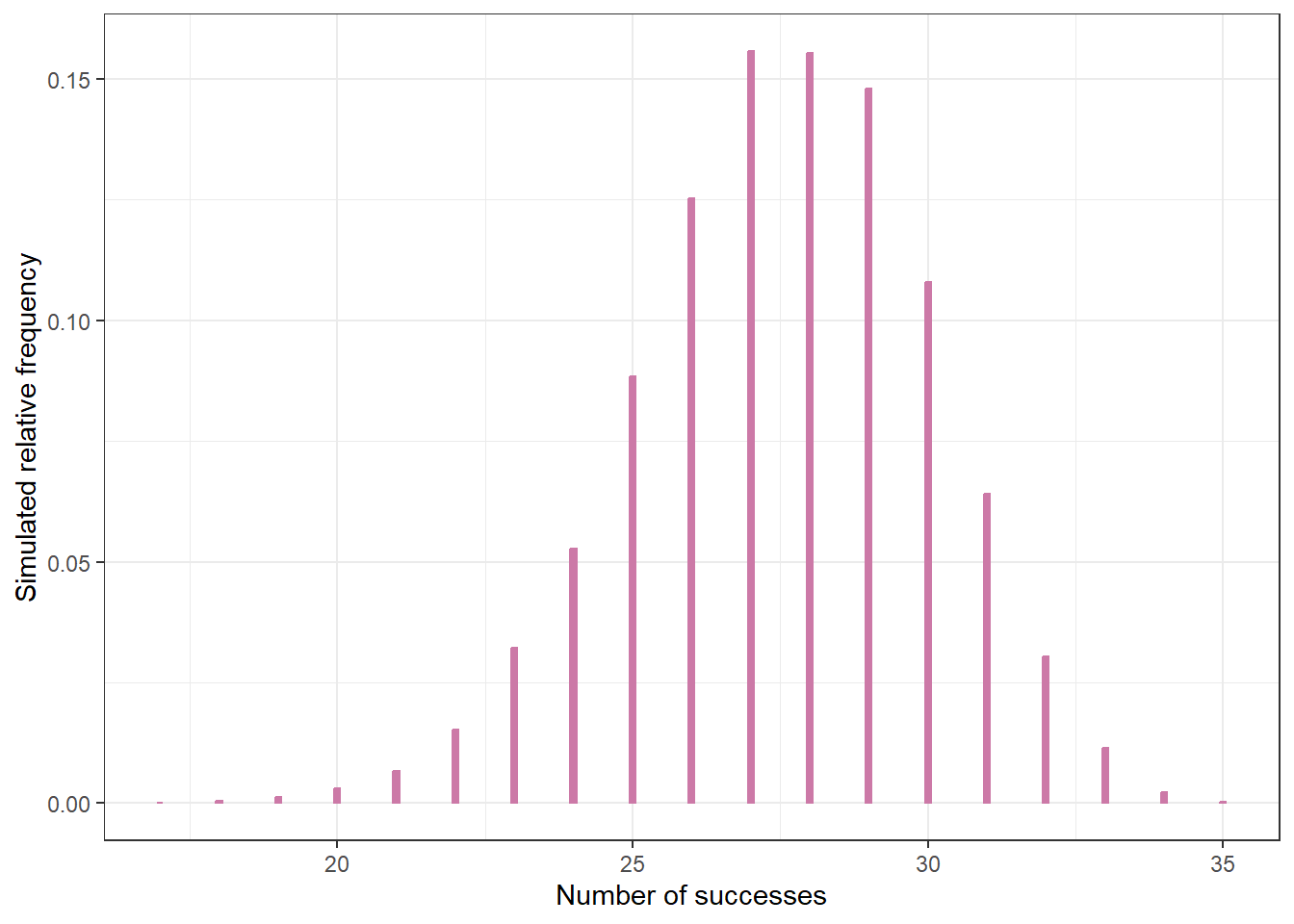

11.3.3 Posterior predictive checking: Free throws

theta = seq(0, 1, 0.0001)

# prior
prior = rep(1, length(theta))
prior = prior / sum(prior)

# data
n = 20 # sample size
y = 10 # sample count of success

# likelihood, assuming binomial
likelihood = dbinom(y, n, theta) # function of theta

# posterior
product = likelihood * prior
posterior = product / sum(product)

Simulate a value of \(\theta\) from its posterior distribution (computed above).
Given \(\theta\), simulate a sequence of 20 independent success/failure trials with probability of success \(\theta\) on each trial. Compute the number of switches for the sequence. (Since we’re interested in the number of switches, we have to generate the individual success/failure results, and not just the total number of successes).
Repeat many times, recording the total number of switches each time. Summarize the values to approximate the posterior predictive distribution of the number of switches.
Compare the observed number of switches (1) to the posterior predictive distribution.

# predictive simulation

n_rep = 10000

switches_sim = rep(NA, n_rep)

for (r in 1:n_rep){
  # simulate a value of theta from its posterior
  theta_sim = sample(theta, 1, replace = TRUE, prob = posterior)
  
  # simulate n independent 1/0 trials with probaility theta
  trials_sim = rbinom(n, 1, theta_sim)
  
  # compute the number of switches using built in r function "rle"
  switches_sim[r] = length(rle(trials_sim)$lengths) - 1
}

ggplot(data.frame(switches_sim),
       aes(x = switches_sim)) +
  geom_bar(aes(y = after_stat(prop)),
           col = bayes_col["posterior_predict"],
           fill = bayes_col["posterior_predict"],
           width = 0.1) +
  labs(x = "Number of switches",
       y = "Simulated relative frequency") +
  theme_bw()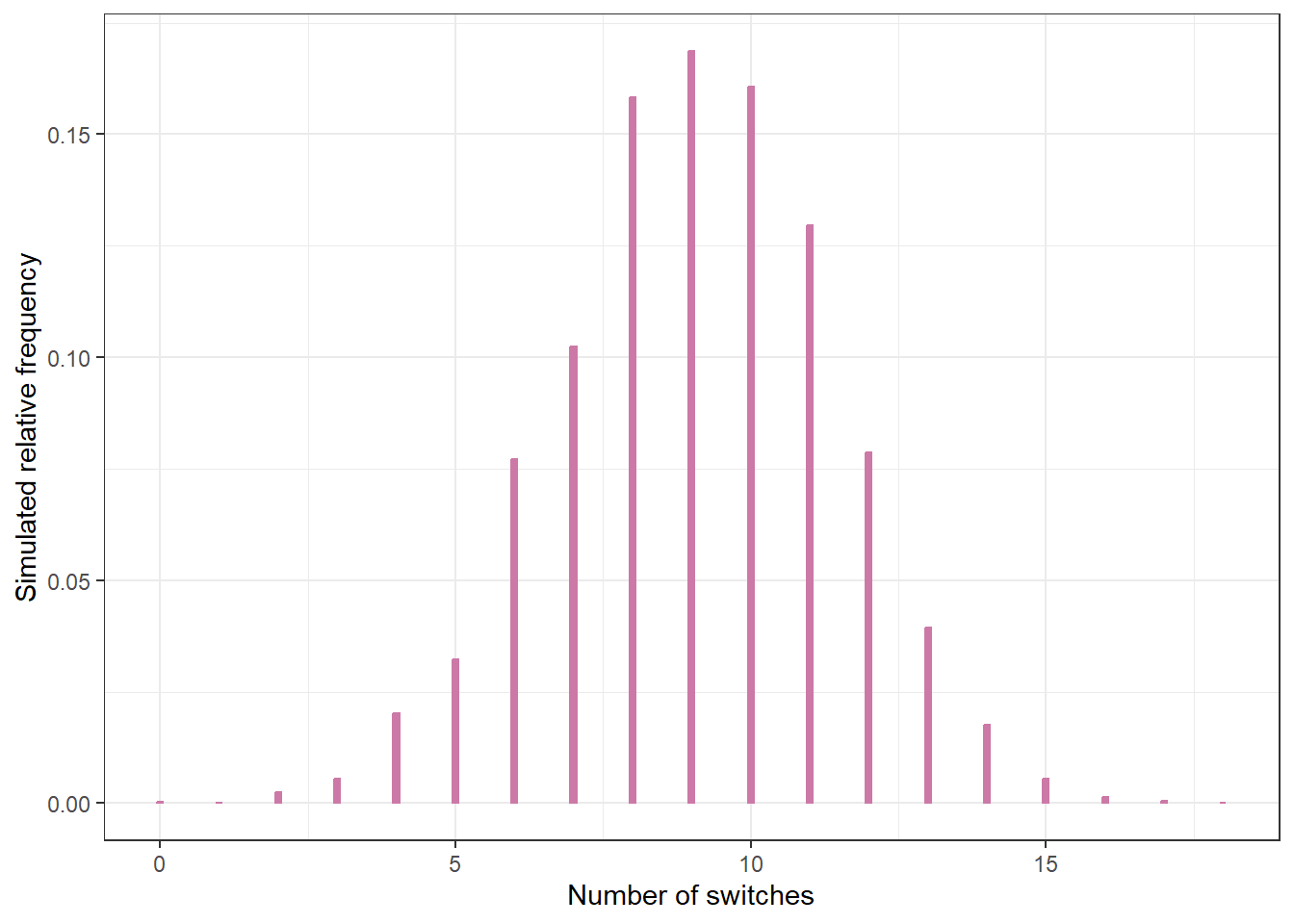

We’ll discuss some problems with this approach later.↩︎