Example 8.1 Assume body temperatures (degrees Fahrenheit) of healthy adults follow a Normal distribution with unknown mean \(\theta\) and known standard deviation \(\sigma=1\). (It’s unrealistic to assume the population standard deviation is known. We’ll consider the case of unknown standard deviation later.) Suppose we wish to estimate \(\theta\), the population mean healthy human body temperature.
If \(\theta\) was known (say \(\theta = 98.6\)), what would the distribution of \(y\) look like? What are some of its features? What does the standard deviation \(\sigma=1\) represent?
Sketch your prior distribution for \(\theta\). What is your single most plausible value for \(\theta\)? About what range of values accounts for most (say 98%) of your prior plausibility? Roughly, what is your prior standard deviation? What does your prior standard deviation represent?
Be careful to distinguish between
Example 8.2 Continuing Example 8.1. Assume first a discrete prior distribution for \(\theta\) which places probability 0.10, 0.25, 0.30, 0.25, 0.10 on the values 97.6, 98.1, 98.6, 99.1, 99.6, respectively.
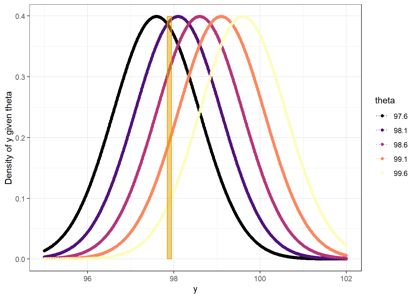
Suppose a single temperature value of 97.9 is observed. Construct a Bayes table and find the posterior distribution of \(\theta\). In particular, how do you determine the likelihood?
Now suppose a second temperature value, 97.5, is observed, independently of the first. Construct a Bayes table and find the posterior distribution of \(\theta\) after observing these two measurements, using the posterior distribution from the previous part as the prior distribution in this part.
Now consider the original prior again. Determine the likelihood of observing temperatures of 97.9 and 97.5 in a sample of size 2. Then construct a Bayes table, starting with the original prior, and find the posterior distribution of \(\theta\) after observing these two measurements. Compare to the previous part.
Consider the original prior again. Suppose that we take a random sample of two temperature measurements, but instead of observing the two individual values, we only observe that the sample mean is 97.7. Determine the likelihood of observing a sample mean of 97.7 in a sample of size 2. (Hint: if \(\bar{y}\) is the sample mean of \(n\) values from a \(N(\theta, \sigma)\) distribution, what is the distribution of \(\bar{y}\)?) Then construct a Bayes table and find the posterior distribution of \(\theta\) after observing this sample mean 97.7. Compare to the previous part.
Example 8.3 Continuing Example 8.1. We’ll now use a grid approximation and assume that any multiple of 0.0001 between 96.0 and 100.0 is a possible value of \(\theta\): 96.0, 96.0001, 96.0002, \(\ldots\), 99.9999, 100.0.
Suppose that the sample mean temperature is \(\bar{y}=97.7\) in a sample of \(n=2\) temperature measurements.
Assume a discrete uniform prior distribution over \(\theta\) values in the grid. Use software to plot the prior distribution, the (scaled) likelihood function, and then find the posterior and plot it. Describe the posterior distribution. What does it say about \(\theta\)?
Assume a discrete triangular prior distribution which is proportional to \(2 - |\theta - 98.0|\) over \(\theta\) values in the grid. Use software to plot the prior distribution, the (scaled) likelihood function, and then find the posterior and plot it. Describe the posterior distribution. What does it say about \(\theta\)?
Now assume a prior distribution which is proportional to a Normal distribution with mean 98.6 and standard deviation 0.7 over \(\theta\) values in the grid. (Careful: be sure not to confuse a Normal prior distribution with the likelihood.) Use software to plot the prior distribution, the (scaled) likelihood function, and then find the posterior and plot it. Describe the posterior distribution. What does it say about \(\theta\)?
Compare the posterior distributions corresponding to the different priors. How does each posterior distribution compare to the prior and the likelihood? Comment on the influence that the prior distribution has. (But remember, this is only a sample of size \(n=2\).)
Example 8.4 Continuing Example 8.1. In a recent study1, the sample mean body temperature in a sample of 208 healthy adults was 97.7 degrees F.
We’ll again use a grid approximation and assume that any multiple of 0.0001 between 96.0 and 100.0 is a possible value of \(\theta\): \(96.0, 96.0001, 96.0002, \ldots, 99.9999, 100.0\).
Assume a discrete uniform prior distribution over \(\theta\) values in the grid. Use software to plot the prior distribution, the (scaled) likelihood function, and then find the posterior and plot it. Describe the posterior distribution. What does it say about \(\theta\)?
Assume a discrete triangular prior distribution which is proportional to \(2 - |\theta - 98.0|\) over \(\theta\) values in the grid. Use software to plot the prior distribution, the (scaled) likelihood function, and then find the posterior and plot it. Describe the posterior distribution. What does it say about \(\theta\)?
Now assume a prior distribution which is proportional to a Normal distribution with mean 98.6 and standard deviation 0.7 over \(\theta\) values in the grid. (Careful: be sure not to confuse a Normal prior distribution with the likelihood.) Use software to plot the prior distribution, the (scaled) likelihood function, and then find the posterior and plot it. Describe the posterior distribution. What does it say about \(\theta\)?
Compare the posterior distributions corresponding to the three different priors. How does each posterior distribution compare to the prior and the likelihood? Comment on the influence that the prior distribution has; how does this compare to the \(n=2\) situation?
The posterior distribution is approximately Normal with posterior mean 97.71 and posterior SD 0.07. Explain what the posterior SD represents.
Compute and interpret in context the posterior probability that \(\theta\) is less than 98.6. Compare to the prior probability.
Compute and interpret in context 50%, 80%, and 98% central posterior credible intervals for \(\theta\). Compare to the prior intervals.
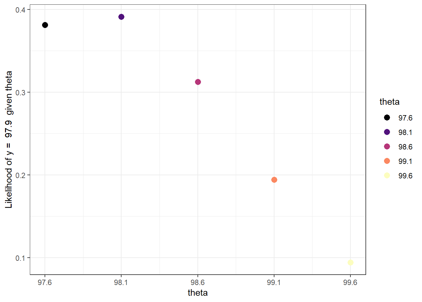
The likelihood is determined by evaluating the Normal(\(\theta\), 1) density at \(y=97.9\) for different values of \(\theta\): dnorm(97.9, theta, 1) or
\[ f(97.9|\theta) = \frac{1}{\sqrt{2\pi}}\,\exp\left(-\frac{1}{2}\left(\frac{97.9-\theta}{1}\right)^2\right) \]
For example, the likelihood for \(\theta = 98.6\) is
\[ \frac{1}{\sqrt{2\pi}}\,\exp\left(-\frac{1}{2}\left(\frac{97.9-98.6}{1}\right)^2\right), \]
or dnorm(97.9, 98.6, 1) = 0.312.
# possible values of theta
theta = seq(97.6, 99.6, 0.5)

# prior
prior = c(0.10, 0.25, 0.30, 0.25, 0.10)
prior = prior / sum(prior)

# observed data
y = 97.9 # single observed value
sigma = 1 # assumed known population SD

# likelihood of observed data for each theta
likelihood = dnorm(y, theta, sigma)

# posterior is proportional to product of prior and likelihood
product = prior * likelihood
posterior = product / sum(product)

bayes_table = data.frame(theta,
                         prior,
                         likelihood,
                         product,
                         posterior)

bayes_table |>
  adorn_totals("row") |>
  kbl(digits = 4) |>
kable_styling()| theta | prior | likelihood | product | posterior |
|---|---|---|---|---|
| 97.6 | 0.10 | 0.3814 | 0.0381 | 0.1326 |
| 98.1 | 0.25 | 0.3910 | 0.0978 | 0.3400 |
| 98.6 | 0.30 | 0.3123 | 0.0937 | 0.3258 |
| 99.1 | 0.25 | 0.1942 | 0.0485 | 0.1688 |
| 99.6 | 0.10 | 0.0940 | 0.0094 | 0.0327 |
| Total | 1.00 | 1.3729 | 0.2875 | 1.0000 |
The likelihood is determined by evaluating the Normal(\(\theta\), 1) density at \(y=97.5\) for different values of \(\theta\): dnorm(97.5, theta, 1) or
\[ f(97.5|\theta) = \frac{1}{\sqrt{2\pi}}\,\exp\left(-\frac{1}{2}\left(\frac{97.5-\theta}{1}\right)^2\right) \]
For example, the likelihood for \(\theta = 98.6\) is
\[ \frac{1}{\sqrt{2\pi}}\,\exp\left(-\frac{1}{2}\left(\frac{97.5-98.6}{1}\right)^2\right), \]
or dnorm(97.5, 98.6, 1) = 0.218.
# prior is posterior from previous part
prior = posterior

# data
y = 97.5 # second observed value

# likelihood of observed data for each theta
likelihood = dnorm(y, theta, sigma)

# posterior is proportional to product of prior and likelihood
product = likelihood * prior
posterior = product / sum(product)

# bayes table
bayes_table = data.frame(theta,
                         prior,
                         likelihood,
                         product,
                         posterior)

bayes_table |>
  adorn_totals("row") |>
  kbl(digits = 4) |>
kable_styling()| theta | prior | likelihood | product | posterior |
|---|---|---|---|---|
| 97.6 | 0.1326 | 0.3970 | 0.0527 | 0.2048 |
| 98.1 | 0.3400 | 0.3332 | 0.1133 | 0.4407 |
| 98.6 | 0.3258 | 0.2179 | 0.0710 | 0.2761 |
| 99.1 | 0.1688 | 0.1109 | 0.0187 | 0.0728 |
| 99.6 | 0.0327 | 0.0440 | 0.0014 | 0.0056 |
| Total | 1.0000 | 1.1029 | 0.2571 | 1.0000 |
Since the two measurements are independent, the likelihood is the product of the likelihoods for \(y=97.9\) and \(y=97.5\): dnorm(97.9, theta, 1) * dnorm(97.5, theta, 1) or
\[ f((97.9, 97.5)|\theta) = \left(\frac{1}{\sqrt{2\pi}}\,\exp\left(-\frac{1}{2}\left(\frac{97.9-\theta}{1}\right)^2\right)\right)\left(\frac{1}{\sqrt{2\pi}}\,\exp\left(-\frac{1}{2}\left(\frac{97.5-\theta}{1}\right)^2\right)\right) \]
For example, the likelihood for \(\theta = 98.6\) is
\[ f((97.9, 97.5)|\theta=98.6) = \left(\frac{1}{\sqrt{2\pi}}\,\exp\left(-\frac{1}{2}\left(\frac{97.9-98.6}{1}\right)^2\right)\right)\left(\frac{1}{\sqrt{2\pi}}\,\exp\left(-\frac{1}{2}\left(\frac{97.5-98.6}{1}\right)^2\right)\right) \]
or dnorm(97.9, 98.6, 1) * dnorm(97.5, 98.6, 1) = (0.312)(0.218) = 0.068.
# prior
prior = c(0.10, 0.25, 0.30, 0.25, 0.10)
prior = prior / sum(prior)

# data
y = c(97.9, 97.5) # two observed values
sigma = 1


# likelihood - function of theta
likelihood = dnorm(y[1], theta, sigma) * dnorm(y[2], theta, sigma)

# posterior
product = likelihood * prior
posterior = product / sum(product)

# bayes table
bayes_table = data.frame(theta,
                         prior,
                         likelihood,
                         product,
                         posterior)

bayes_table |>
  adorn_totals("row") |>
  kbl(digits = 4) |>
kable_styling()| theta | prior | likelihood | product | posterior |
|---|---|---|---|---|
| 97.6 | 0.10 | 0.1514 | 0.0151 | 0.2048 |
| 98.1 | 0.25 | 0.1303 | 0.0326 | 0.4407 |
| 98.6 | 0.30 | 0.0680 | 0.0204 | 0.2761 |
| 99.1 | 0.25 | 0.0215 | 0.0054 | 0.0728 |
| 99.6 | 0.10 | 0.0041 | 0.0004 | 0.0056 |
| Total | 1.00 | 0.3754 | 0.0739 | 1.0000 |
For a sample of size \(n\) from a \(N(\theta,\sigma)\) distribution, the sample mean \(\bar{y}\) follows a \(N\left(\theta, \frac{\sigma}{\sqrt{n}}\right)\) distribution. Remember: \(\sigma/\sqrt{n}\) represents the sample-to-sample variability of sample means.
The likelihood is determined by evaluating the Normal(\(\theta\), \(\frac{1}{\sqrt{2}}\)) density at \(\bar{y}=97.7\) for different values of \(\theta\): dnorm(97.7, theta, 1 / sqrt(2)) or
\[ f_{\bar{Y}}(97.7|\theta) \propto \exp\left(-\frac{1}{2}\left(\frac{97.7-\theta}{1/\sqrt{2}}\right)^2\right) \]
For example, the likelihood for \(\theta = 98.6\) is
\[ f_{\bar{Y}}((97.7)|\theta=98.6) \propto \exp\left(-\frac{1}{2}\left(\frac{97.7-98.6}{1/\sqrt{2}}\right)^2\right) \]
or dnorm(97.7, 98.6, 1 / sqrt(2)) = 0.251.
The likelihood is not the same as in the previous part. There are many samples with a sample mean of 97.7, of which the sample (97.9, 97.5) is only one possibility, so the likelihood of observing a sample mean of 97.7 is greater than the likelihood of (97.9, 97.5). However, while the likelihood is not the same as in the previous part, it is proportionally the same. That is, the likelihood in this part has the same shape as the likelihood in the previous part. For example, the ratio of the likelihoods for \(\theta=98.6\) and \(\theta=98.1\) is the same in both parts: \(0.4808/0.2510 = 1.91\) and \(0.1303/0.068=1.91\). Since the prior distribution is the same in both parts, and the likelihoods are proportionally the same, then the posterior distributions are the same.
# prior
prior = c(0.10, 0.25, 0.30, 0.25, 0.10)
prior = prior / sum(prior)

# data
n = 2
y = 97.7 # sample mean
sigma = 1


# likelihood
likelihood = dnorm(y, theta, sigma / sqrt(n)) # function of theta

# posterior
product = likelihood * prior
posterior = product / sum(product)

# bayes table
bayes_table = data.frame(theta,
                         prior,
                         likelihood,
                         product,
                         posterior)

bayes_table |>
  adorn_totals("row") |>
  kbl(digits = 4) |>
kable_styling()| theta | prior | likelihood | product | posterior |
|---|---|---|---|---|
| 97.6 | 0.10 | 0.5586 | 0.0559 | 0.2048 |
| 98.1 | 0.25 | 0.4808 | 0.1202 | 0.4407 |
| 98.6 | 0.30 | 0.2510 | 0.0753 | 0.2761 |
| 99.1 | 0.25 | 0.0795 | 0.0199 | 0.0728 |
| 99.6 | 0.10 | 0.0153 | 0.0015 | 0.0056 |
| Total | 1.00 | 1.3851 | 0.2727 | 1.0000 |
The only change is the grid and the prior.
theta = seq(96, 100, 0.0001)

# prior
prior = rep(1, length(theta)) # shape of prior
prior = prior / sum(prior) # scales so that prior sums to 1

# data
n = 2 # sample size
y = 97.7 # sample mean
sigma = 1 # assumed known

# likelihood
likelihood = dnorm(y, theta, sigma / sqrt(n)) # function of theta

# posterior
product = likelihood * prior
posterior = product / sum(product)

bayes_table = data.frame(theta,
                         prior,
                         likelihood,
                         product,
                         posterior)
bayes_table |>
# scale likelihood for plotting only
mutate(likelihood = likelihood / sum(likelihood)) |>
select(theta, prior, likelihood, posterior) |>
pivot_longer(!theta,
names_to = "source",
values_to = "probability") |>
mutate(source = fct_relevel(source, "prior", "likelihood", "posterior")) |>
ggplot(aes(x = theta,
y = probability,
col = source)) +
geom_line(aes(linetype = source), linewidth = 1) +
scale_color_manual(values = bayes_col) +
scale_linetype_manual(values = bayes_lty) +
theme_bw() +
# remove y-axis labels
theme(axis.title.y = element_blank(),
axis.text.y = element_blank(),
axis.ticks.y = element_blank())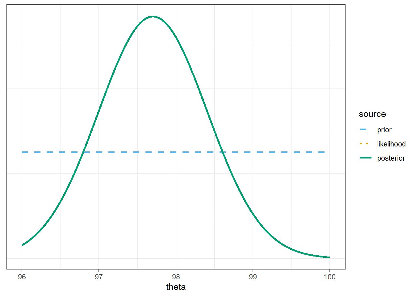
The only change is the prior
theta = seq(96, 100, 0.0001)

# prior
prior = 2 - abs(theta - 98) # shape of prior
prior = prior / sum(prior) # scales so that prior sums to 1

# data
n = 2 # sample size
y = 97.7 # sample mean
sigma = 1 # assumed known

# likelihood
likelihood = dnorm(y, theta, sigma / sqrt(n)) # function of theta

# posterior
product = likelihood * prior
posterior = product / sum(product)

bayes_table = data.frame(theta,
                         prior,
                         likelihood,
                         product,
                         posterior)
bayes_table |>
# scale likelihood for plotting only
mutate(likelihood = likelihood / sum(likelihood)) |>
select(theta, prior, likelihood, posterior) |>
pivot_longer(!theta,
names_to = "source",
values_to = "probability") |>
mutate(source = fct_relevel(source, "prior", "likelihood", "posterior")) |>
ggplot(aes(x = theta,
y = probability,
col = source)) +
geom_line(aes(linetype = source), linewidth = 1) +
scale_color_manual(values = bayes_col) +
scale_linetype_manual(values = bayes_lty) +
theme_bw() +
# remove y-axis labels
theme(axis.title.y = element_blank(),
axis.text.y = element_blank(),
axis.ticks.y = element_blank())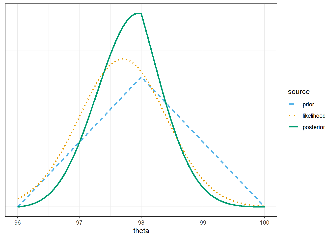
The only change is the prior
theta = seq(96, 100, 0.0001)

# prior
prior = dnorm(theta, 98.6, 0.7) # shape of prior
prior = prior / sum(prior) # scales so that prior sums to 1

# data
n = 2 # sample size
y = 97.7 # sample mean
sigma = 1 # assumed known

# likelihood
likelihood = dnorm(y, theta, sigma / sqrt(n)) # function of theta

# posterior
product = likelihood * prior
posterior = product / sum(product)

bayes_table = data.frame(theta,
                         prior,
                         likelihood,
                         product,
                         posterior)
bayes_table |>
# scale likelihood for plotting only
mutate(likelihood = likelihood / sum(likelihood)) |>
select(theta, prior, likelihood, posterior) |>
pivot_longer(!theta,
names_to = "source",
values_to = "probability") |>
mutate(source = fct_relevel(source, "prior", "likelihood", "posterior")) |>
ggplot(aes(x = theta,
y = probability,
col = source)) +
geom_line(aes(linetype = source), linewidth = 1) +
scale_color_manual(values = bayes_col) +
scale_linetype_manual(values = bayes_lty) +
theme_bw() +
# remove y-axis labels
theme(axis.title.y = element_blank(),
axis.text.y = element_blank(),
axis.ticks.y = element_blank())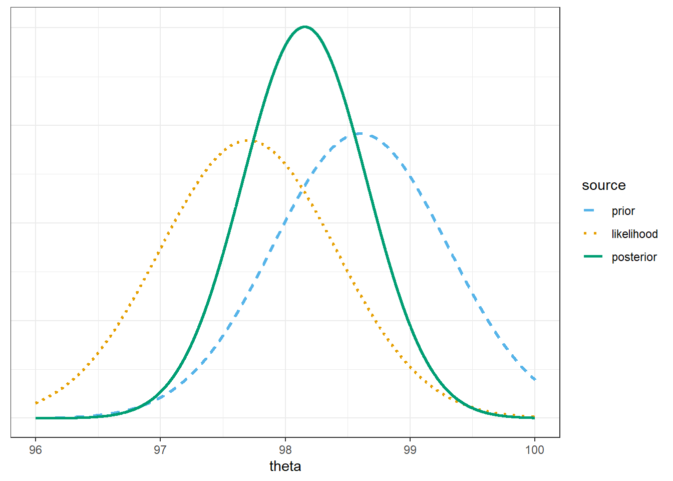
The only change is the data.
theta = seq(96, 100, 0.0001)

# prior
prior = rep(1, length(theta)) # shape of prior
prior = prior / sum(prior) # scales so that prior sums to 1

# data
n = 208 # sample size
y = 97.7 # sample mean
sigma = 1 # assumed known

# likelihood
likelihood = dnorm(y, theta, sigma / sqrt(n)) # function of theta

# posterior
product = likelihood * prior
posterior = product / sum(product)

bayes_table = data.frame(theta,
                         prior,
                         likelihood,
                         product,
                         posterior)
bayes_table |>
# scale likelihood for plotting only
mutate(likelihood = likelihood / sum(likelihood)) |>
select(theta, prior, likelihood, posterior) |>
pivot_longer(!theta,
names_to = "source",
values_to = "probability") |>
mutate(source = fct_relevel(source, "prior", "likelihood", "posterior")) |>
ggplot(aes(x = theta,
y = probability,
col = source)) +
geom_line(aes(linetype = source), linewidth = 1) +
scale_color_manual(values = bayes_col) +
scale_linetype_manual(values = bayes_lty) +
theme_bw() +
# remove y-axis labels
theme(axis.title.y = element_blank(),
axis.text.y = element_blank(),
axis.ticks.y = element_blank())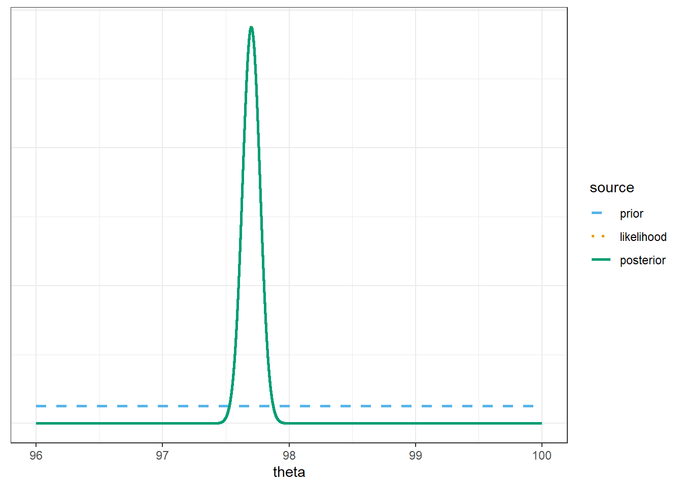
The only change is the prior
theta = seq(96, 100, 0.0001)

# prior
prior = 2 - abs(theta - 98) # shape of prior
prior = prior / sum(prior) # scales so that prior sums to 1

# data
n = 208 # sample size
y = 97.7 # sample mean
sigma = 1 # assumed known

# likelihood
likelihood = dnorm(y, theta, sigma / sqrt(n)) # function of theta

# posterior
product = likelihood * prior
posterior = product / sum(product)

bayes_table = data.frame(theta,
                         prior,
                         likelihood,
                         product,
                         posterior)
bayes_table |>
# scale likelihood for plotting only
mutate(likelihood = likelihood / sum(likelihood)) |>
select(theta, prior, likelihood, posterior) |>
pivot_longer(!theta,
names_to = "source",
values_to = "probability") |>
mutate(source = fct_relevel(source, "prior", "likelihood", "posterior")) |>
ggplot(aes(x = theta,
y = probability,
col = source)) +
geom_line(aes(linetype = source), linewidth = 1) +
scale_color_manual(values = bayes_col) +
scale_linetype_manual(values = bayes_lty) +
theme_bw() +
# remove y-axis labels
theme(axis.title.y = element_blank(),
axis.text.y = element_blank(),
axis.ticks.y = element_blank())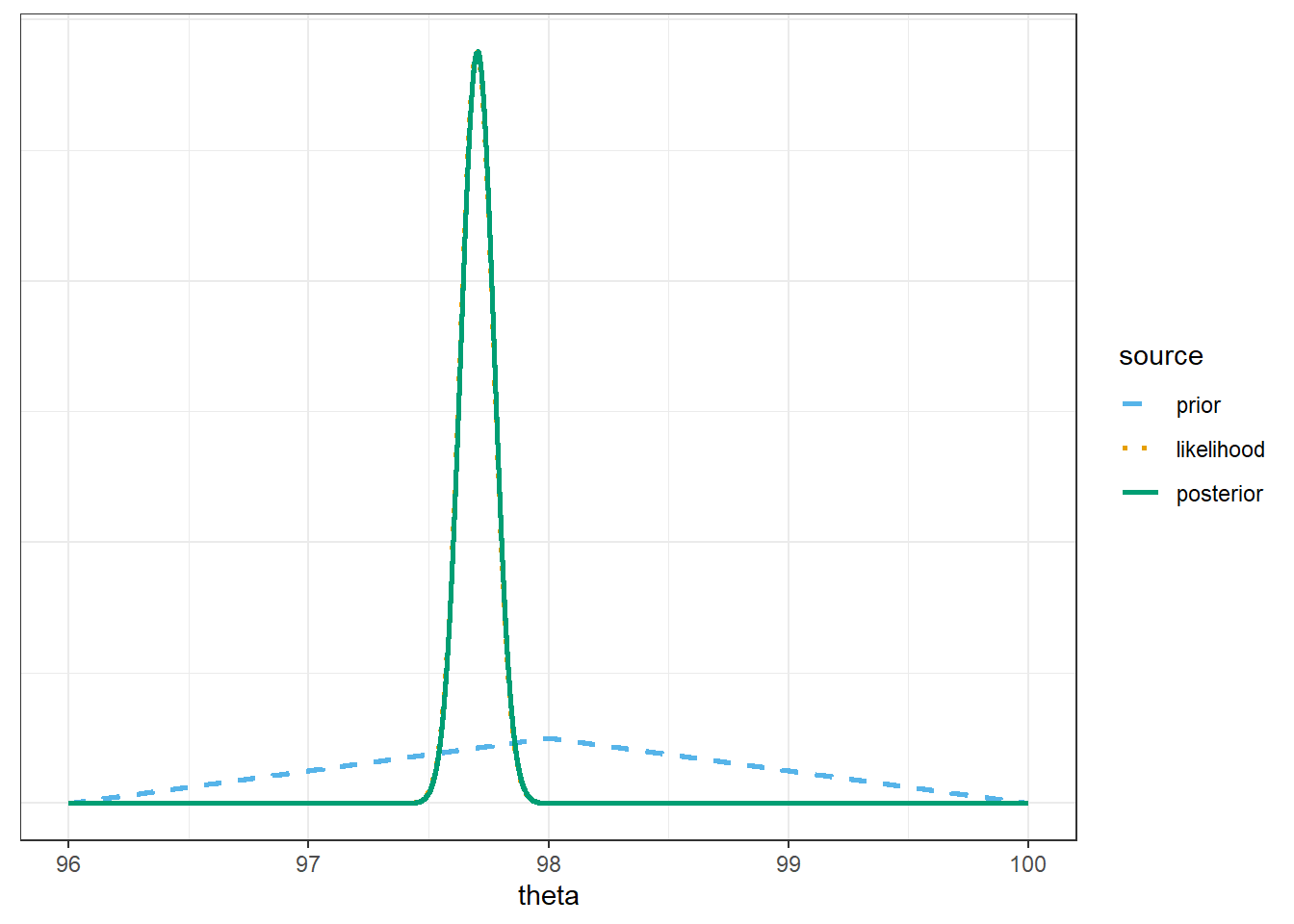
The only change is the prior
theta = seq(96, 100, 0.0001)

# prior
prior = dnorm(theta, 98.6, 0.7) # shape of prior
prior = prior / sum(prior) # scales so that prior sums to 1

# data
n = 208 # sample size
y = 97.7 # sample mean
sigma = 1 # assumed known

# likelihood
likelihood = dnorm(y, theta, sigma / sqrt(n)) # function of theta

# posterior
product = likelihood * prior
posterior = product / sum(product)

bayes_table = data.frame(theta,
                         prior,
                         likelihood,
                         product,
                         posterior)
bayes_table |>
# scale likelihood for plotting only
mutate(likelihood = likelihood / sum(likelihood)) |>
select(theta, prior, likelihood, posterior) |>
pivot_longer(!theta,
names_to = "source",
values_to = "probability") |>
mutate(source = fct_relevel(source, "prior", "likelihood", "posterior")) |>
ggplot(aes(x = theta,
y = probability,
col = source)) +
geom_line(aes(linetype = source), linewidth = 1) +
scale_color_manual(values = bayes_col) +
scale_linetype_manual(values = bayes_lty) +
theme_bw() +
# remove y-axis labels
theme(axis.title.y = element_blank(),
axis.text.y = element_blank(),
axis.ticks.y = element_blank())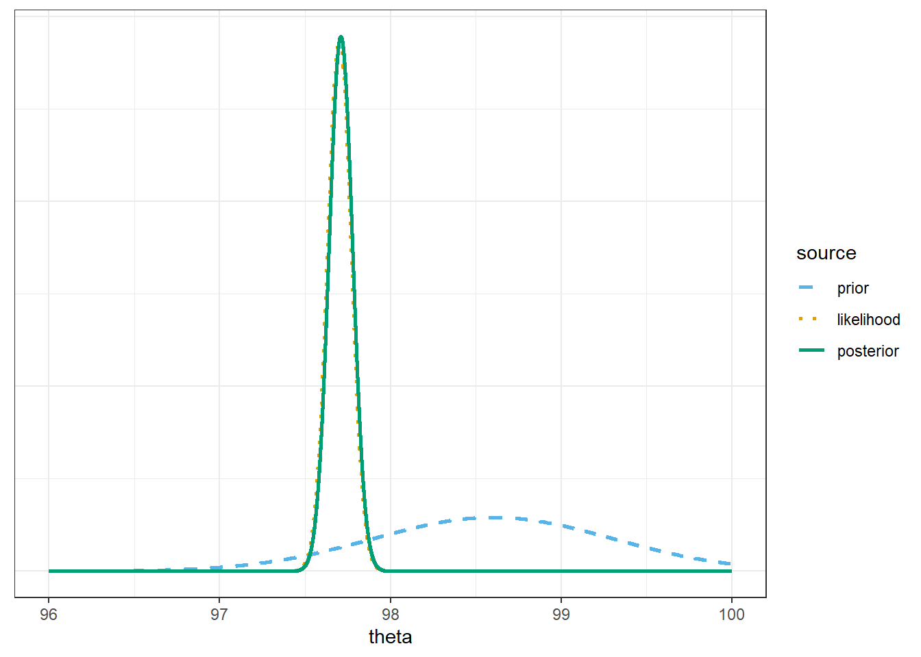
# posterior mean
post_mean = sum(theta * posterior)
post_mean
[1] 97.70874# posterior SD
post_var = sum(theta ^ 2 * posterior) - post_mean ^ 2
post_sd = sqrt(post_var)
post_sd[1] 0.06899985# posterior probability theta is less than 0.7
pnorm(98.6, post_mean, post_sd)[1] 1# endpoints of posterior 50% credible interval
qnorm(c(0.25, 0.75), post_mean, post_sd)[1] 97.66220 97.75528# endpoints of posterior 80% credible interval
qnorm(c(0.10, 0.90), post_mean, post_sd)[1] 97.62032 97.79717# endpoints of posterior 98% credible interval
qnorm(c(0.01, 0.99), post_mean, post_sd)[1] 97.54823 97.86926Source and a related article.↩︎