12 Beta-Binomial Model
- Bayesian analysis is based on the posterior distribution of parameters \(\theta\) given data \(y\).
- The data \(y\) might be discrete (e.g., count data) or continuous (e.g., measurement data).
- However, parameters \(\theta\) almost always take values on a continuous scale, even when the data are discrete.
- Now we introduce continuous prior and posterior distributions to quantify uncertainty about parameters. Some general notation:
- \(\theta\) represents1 parameters of interest usually taking values on a continuous scale
- \(y\) denotes observed sample data2 (discrete or continuous)
- \(\pi(\theta)\) denotes the prior distribution of \(\theta\), usually a probability density function (pdf) over possible values of \(\theta\)
- \(f(y|\theta)\) denotes the likelihood function, a function of continuous \(\theta\) for fixed \(y\)
- \(\pi(\theta |y)\) denotes the posterior distribution of \(\theta\), the conditional distribution of \(\theta\) given the data \(y\).
- Bayes rule works analogously for a continuous parameter \(\theta\), given data \(y\) \[\begin{align*} \pi(\theta|y) & = \frac{f(y|\theta)\pi(\theta)}{f(y)}\\ & \\ \pi(\theta|y) & \propto f(y|\theta)\pi(\theta)\\ & \\ \text{posterior} & \propto \text{likelihood}\times \text{prior} \end{align*}\]
- Predictive distribution can be found using a continuous analog of the law of total probability \[\begin{align*} \text{Prior predictive} & & f(y) & = \int_{-\infty}^{\infty}f(y|\theta)\pi(\theta) d\theta,\\ \text{Posterior predictive} & & f(\tilde{y}|\theta) & = \int_{-\infty}^{\infty}f(\tilde{y}|\theta)\pi(\theta|y) d\theta. \end{align*}\] However, we almost always use simulation to approximate predictive distributions.
Example 12.1 Recall Example 10.4 which concerned \(\theta\), the population proportion of students in Cal Poly statistics classes who prefer to consider data as a singular noun (as in “the data is”).
Why might we not want to assume a Normal prior distribution for \(\theta\)?
In Example 10.4 we assumed a prior distribution for \(\theta\) which is proportional to \(\theta^2,\; 0<\theta<1\). In that example, we used a grid approximation for the prior distribution, but now we’ll treat the distribution as continuous. Sketch this prior distribution.
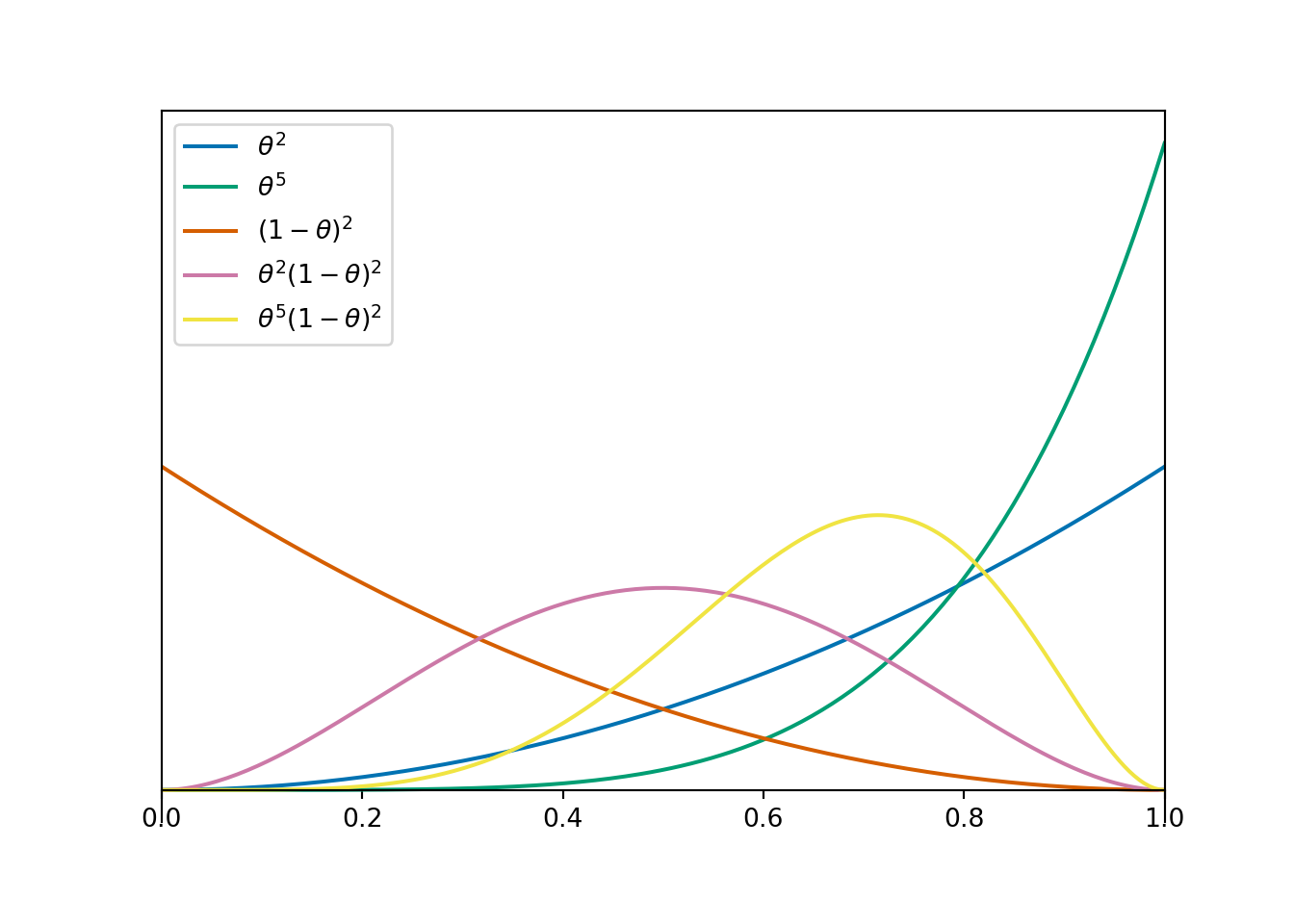
Now we’ll consider a few more prior distributions. Sketch each of the following priors. How do they compare?
- proportional to \(\theta^2,\; 0<\theta<1\). (from previous)
- proportional to \(\theta^5,\; 0<\theta<1\).
- proportional to \((1-\theta)^2,\; 0<\theta<1\).
- proportional to \(\theta^2(1-\theta)^2,\; 0<\theta<1\).
- proportional to \(\theta^5(1-\theta)^2,\; 0<\theta<1\).
- A continuous random variable \(U\) has a Beta distribution with shape parameters \(\alpha>0\) and \(\beta>0\) if its density (pdf) satisfies3 \[ p(u) \propto u^{\alpha-1}(1-u)^{\beta-1}, \quad 0<u<1. \]
- If \(\alpha = \beta\) the distribution is symmetric about 0.5
- If \(\alpha > \beta\) the distribution is skewed to the left (with greater density above 0.5 than below)
- If \(\alpha < \beta\) the distribution is skewed to the right (with greater density below 0.5 than above)
- If \(\alpha = 1\) and \(\beta = 1\), the Beta(1, 1) distribution is the Uniform distribution on (0, 1).
- It can be shown that a Beta(\(\alpha\), \(\beta\)) distribution has \[\begin{align*} \text{Mean (EV):} & \quad \frac{\alpha}{\alpha+\beta}\\ \text{Variance:} & \quad \frac{\left(\frac{\alpha}{\alpha+\beta}\right)\left(1-\frac{\alpha}{\alpha+\beta}\right)}{\alpha+\beta+1} \\ \text{Mode:} & \quad \frac{\alpha -1}{\alpha+\beta-2}, \qquad \text{(if $\alpha>1$, $\beta\ge1$ or $\alpha\ge1$, $\beta>1$; otherwise, there is not a unique mode)} \end{align*}\]
Example 12.2 Continuing Example 12.1.
- Each of the distributions in the previous example was a Beta distribution. For each distribution, identify the shape parameters and the prior mean and standard deviation.
| Prior proportional to | Prior \(\alpha\) | Prior \(\beta\) | Prior Mean | Prior SD |
|---|---|---|---|---|
| \(\theta^2\) | ||||
| \(\theta^5\) | ||||
| \((1-\theta)^2\) | ||||
| \(\theta^2(1-\theta)^2\) | ||||
| \(\theta^5(1-\theta)^2\) |
Assume a Beta(3, 1) prior distribution for \(\theta\). Now suppose that 31 students in a sample of 35 Cal Poly statistics students prefer data as singular. Write the function that defines the shape of the likelihood as a function of \(\theta, 0<\theta<1\).
Write the function that defines the shape of the posterior density as a function of \(\theta, 0<\theta<1.\) Is this a Beta distribution? If so, specify the values of \(\alpha\) and \(\beta\).
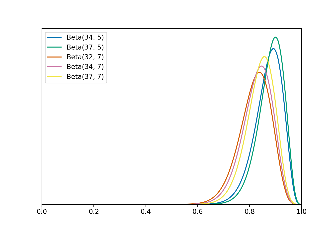
Starting with each of the prior distributions from the first part, find the posterior distribution of \(\theta\) based on this sample, and identify it as a Beta distribution by specifying the shape parameters \(\alpha\) and \(\beta\).
| Prior | Posterior \(\alpha\) | Posterior \(\beta\) | Posterior Mean | Posterior SD |
|---|---|---|---|---|
| Beta(3, 1) | ||||
| Beta(6, 1) | ||||
| Beta(1, 3) | ||||
| Beta(3, 3) | ||||
| Beta(6, 3) |
- For each of the posterior distributions in the previous part, compute the posterior mean and standard deviation. How does each posterior distribution compare to its respective prior distribution?
- Beta-Binomial model. If \(\theta\) has a Beta\((\alpha, \beta)\) prior distribution and the conditional distribution of \(y\) given \(\theta\) is the Binomial\((n, \theta)\) distribution, then the posterior distribution of \(\theta\) given \(y\) is the Beta\((\alpha + y, \beta + n - y)\) distribution4. \[\begin{align*} \text{prior:} & & \pi(\theta) & \propto \theta^{\alpha-1}(1-\theta)^{\beta-1}, \quad 0<\theta<1,\\ \\ \text{likelihood:} & & f(y|\theta) & \propto \theta^y (1-\theta)^{n-y}, \quad 0 < \theta < 1,\\ \\ \text{posterior:} & & \pi(\theta|y) & \propto \theta^{\alpha+y-1}(1-\theta)^{\beta+n-y-1}, \quad 0<\theta<1. \end{align*}\]
- In a sense, you can interpret \(\alpha\) as “prior successes” and \(\beta\) as “prior failures”, but these are only “pseudo-observations”. Also, \(\alpha\) and \(\beta\) are not necessarily integers.
| Prior | Data | Posterior | |
|---|---|---|---|
| Successes | \(\alpha\) | \(y\) | \(\alpha + y\) |
| Failures | \(\beta\) | \(n-y\) | \(\beta + n - y\) |
| Total | \(\alpha+\beta\) | \(n\) | \(\alpha + \beta + n\) |
Example 12.3 In Example 10.4 we essentially assumed a Beta(3, 1) prior but we used grid approximation to compute the posterior. Now we’ll compare our results from that exercise to those using the continuous Beta(3, 1) prior.
Assume that \(\theta\) has a Beta(3, 1) prior distribution and that 31 students in a sample of 35 Cal Poly statistics students prefer data as singular.
Plot the prior distribution, (scaled) likelihood, and posterior distribution.
Use software to find 50%, 80%, and 98% central posterior credible intervals.
Compare the results to those using the grid approximation.
Express the posterior mean as a weighted average of the prior mean and sample proportion. Describe what the weights are, and explain why they make sense.
- In the Beta-Binomial model, the posterior mean \(E(\theta|y)\) can be expressed as a weighted average of the prior mean \(E(\theta)=\frac{\alpha}{\alpha + \beta}\) and the sample proportion \(\hat{p}=y/n\). \[ E(\theta|y) = \frac{\alpha+\beta}{\alpha+\beta+n}E(\theta) + \frac{n}{\alpha+\beta+n}\hat{p} \]
- As more data are collected, more weight is given to the sample proportion (and less weight to the prior mean).
- The prior “weight” is determined by \(\alpha+\beta\), which is sometimes called the concentration and measured in “pseudo-observations”.
- Larger values of \(\alpha+\beta\) indicate stronger prior beliefs, due to smaller prior variance, and give more weight to the prior mean.
- The posterior variance generally gets smaller as more data are collected \[ \text{Var}(\theta |y) = \frac{E(\theta|y)(1-E(\theta|y))}{\alpha+\beta+n+1} \]
Example 12.4 Continuing the previous examples, we’ll now consider predictive distributions. Assume that \(\theta\) has a Beta(3, 1) prior distribution.
Before observing any data, suppose we plan to randomly select a sample of 35 Cal Poly statistics students. Let \(y\) represent the number of students in the selected sample who prefer data as singular. Explain how we could use simulation to approximate the prior predictive distribution of \(y\). Then conduct the simulation and approximate the prior predictive distribution. Is the prior predictive distribution truly discrete or continuous? How does the prior predictive distribution compare to the one from Example 10.4?
Now suppose we observe 31 students in a sample of 35 Cal Poly statistics students prefer data as singular, so that the posterior distribution of \(\theta\) is the Beta(34, 5) distribution. Suppose we plan to randomly select another sample of 35 Cal Poly statistics students. Let \(\tilde{y}\) represent the number of students in the selected sample who prefer data as singular. Explain how we could use simulation to approximate the posterior predictive distribution of \(\tilde{y}\). Then conduct the simulation and approximate the posterior predictive distribution. Is the posterior predictive distribution truly discrete or continuous? How does the posterior predictive distribution compare to the one from Example 10.5?
Use the simulation results to approximate a 95% posterior prediction interval for \(\tilde{y}\). Write a clearly worded sentence interpreting this interval in context.
- You can tune the shape parameters — \(\alpha\) (like “prior successes”) and \(\beta\) (like “prior failures”) — of a Beta distribution to your prior beliefs in a few ways. Recall that \(\kappa = \alpha + \beta\) is the “concentration” or “equivalent prior sample size”.
- If prior mean \(\mu\) and prior concentration \(\kappa\) are specified then \[\begin{align*} \alpha &= \mu \kappa\\ \beta & =(1-\mu)\kappa \end{align*}\]
- If prior mode \(\omega\) and prior concentration \(\kappa\) (with \(\kappa>2\)) are specified then \[\begin{align*} \alpha &= \omega (\kappa-2) + 1\\ \beta & = (1-\omega) (\kappa-2) + 1 \end{align*}\]
- If prior mean \(\mu\) and prior sd \(\sigma\) are specified then \[\begin{align*} \alpha &= \mu\left(\frac{\mu(1-\mu)}{\sigma^2} -1\right)\\ \beta & = \left(1-\mu\right)\left(\frac{\mu(1-\mu)}{\sigma^2} -1\right) %\beta & = \alpha\left(\frac{1}{\mu} - 1\right)\\ \end{align*}\]
- You can also specify two percentiles and use software to find \(\alpha\) and \(\beta\). For example, you could specify the endpoints of a prior 98% credible interval.
12.1 Notes
12.1.1 Prior Beta distributions
| Distribution | \(\alpha\) | \(\beta\) | Proportional to | Mean | SD | |
|---|---|---|---|---|---|---|
| a | Beta(3, 1) | 3 | 1 | \(\theta^2, 0<\theta < 1\) | 0.750 | 0.194 |
| b | Beta(6, 1) | 6 | 1 | \(\theta^5, 0<\theta < 1\) | 0.857 | 0.124 |
| c | Beta(1, 3) | 1 | 3 | \((1-\theta)^2, 0<\theta < 1\) | 0.250 | 0.194 |
| d | Beta(3, 3) | 3 | 3 | \(\theta^2(1-\theta)^2, 0<\theta < 1\) | 0.500 | 0.189 |
| e | Beta(6, 3) | 6 | 3 | \(\theta^5(1-\theta)^2, 0<\theta < 1\) | 0.667 | 0.149 |
12.1.2 Posterior Beta distributions
| Prior Distribution | Posterior proportional to | Posterior Distribution | Posterior Mean | Posterior SD | |
|---|---|---|---|---|---|
| a | Beta(3, 1) | \(\theta^{2 + 31}(1-\theta)^{0 + 4}, 0 < \theta < 1\) | Beta(34, 5) | 0.872 | 0.053 |
| b | Beta(6, 1) | \(\theta^{5 + 31}(1-\theta)^{0 + 4}, 0 < \theta < 1\) | Beta(37, 5) | 0.881 | 0.049 |
| c | Beta(1, 3) | \(\theta^{0 + 31}(1-\theta)^{2 + 4}, 0 < \theta < 1\) | Beta(32, 7) | 0.821 | 0.061 |
| d | Beta(3, 3) | \(\theta^{2 + 31}(1-\theta)^{2 + 4}, 0 < \theta < 1\) | Beta(34, 7) | 0.829 | 0.058 |
| e | Beta(6, 3) | \(\theta^{5 + 31}(1-\theta)^{2 + 4}, 0 < \theta < 1\) | Beta(37, 7) | 0.841 | 0.055 |
12.1.3 Posterior distribution
The Beta(3, 1) prior is proportional to \[ \pi(\theta) \propto \theta^{3 - 1}(1-\theta)^{1-1}, \qquad 0 < \theta < 1. \]
Given \(\theta\), the number of students in the sample who prefer data as singular, \(y\), follows a Binomial(35, \(\theta\)) distribution. The likelihood is the probability of observing \(y=31\) viewed as a function of \(\theta\). \[\begin{align*} f(31|\theta) & = \binom{35}{31}\theta^{31}(1-\theta)^4, \qquad 0 < \theta <1\\ & \propto \theta^{31}(1-\theta)^4, \qquad 0 < \theta <1 \end{align*}\] The constant \(\binom{35}{31}\) does not affect the shape of the likelihood as a function of \(\theta\).
The posterior density, as a function of \(\theta\), is proportional to \[\begin{align*} \pi(\theta|y = 31) & \propto \left(\theta^2\right)\left(\theta^{31}(1-\theta)^4\right), \qquad 0 <\theta < 1\\ & \propto \theta^{33}(1-\theta)^4, \qquad 0 <\theta < 1\\ & \propto \theta^{34 - 1}(1-\theta)^{5 - 1}, \qquad 0 <\theta < 1\\ \end{align*}\] Therefore, the posterior distribution of \(\theta\) is the Beta(3 + 31, 1 + 35 - 31), that is, the Beta(34, 5) distribution.
We can use stat_fun to plot a function over a range. This works fine for the dbeta prior and posterior, but unfortunately the likeihood, determined by dbinom is not on a density scale.
# Beta prior
alpha_prior = 3
beta_prior = 1

# data
n = 35
y = 31

# Beta posterior
alpha_post = alpha_prior + y
beta_post = beta_prior + n - y

# Plot
ggplot(data.frame(x = c(0, 1)),
       aes(x = x)) +
  # prior
  stat_function(fun = dbeta,
                args = list(shape1 = alpha_prior,
                            shape2 = beta_prior),
                col = bayes_col["prior"],
                lty = bayes_lty["prior"],
                linewidth = 1) +
  # likelihood
  stat_function(fun = dbinom,
                args = list(size = n,
                            x = y),
                col = bayes_col["likelihood"],
                lty = bayes_lty["likelihood"],
                linewidth = 1) +
  # posterior
  stat_function(fun = dbeta,
                args = list(shape1 = alpha_post,
                            shape2 = beta_post),
                col = bayes_col["posterior"],
                lty = bayes_lty["posterior"],
                linewidth = 1) +
  labs(x = "theta",
       y = "") +
  theme_bw()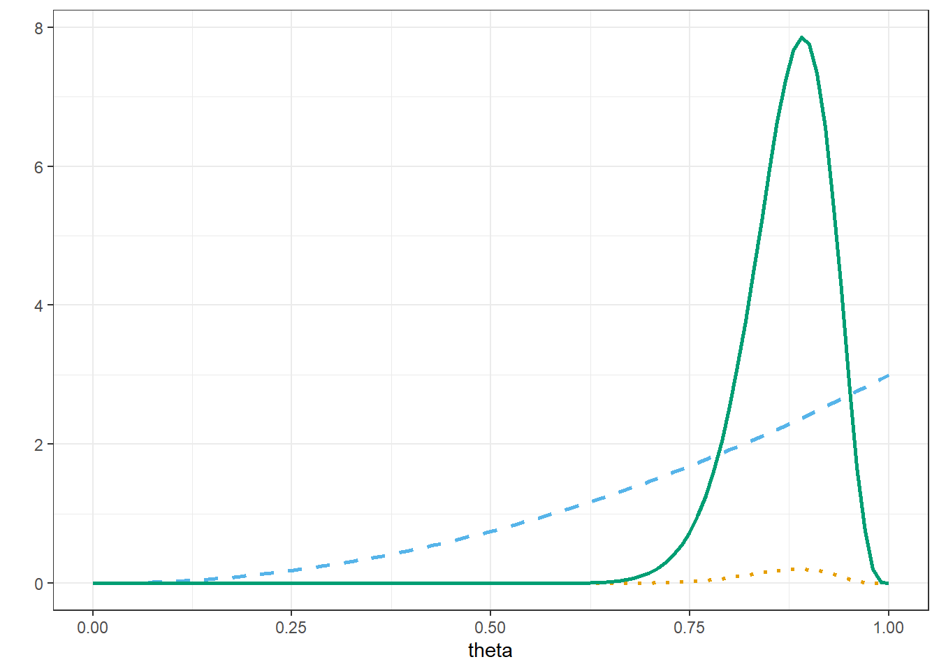
The following code creates a scaled version of the likelihood function for plotting (and moves a few things around to create a legend).
# data
n = 35
y = 31

# scaled likelihood, depends on data: n, y
likelihood_scaled <- function(theta) {
  likelihood <- function(theta) {
    dbinom(x = y, size = n, prob = theta)
  }
  scaling_constant <- integrate(likelihood, lower = 0, upper = 1)[[1]]
  likelihood(theta) / scaling_constant
}

# Plot
ggplot(data.frame(x = c(0, 1)),
       aes(x = x)) +
  # prior
  stat_function(fun = dbeta,
                args = list(shape1 = alpha_prior,
                            shape2 = beta_prior),
                lty = bayes_lty["prior"],
                linewidth = 1,
                aes(color = "prior", linetype = "prior")) +
  # (scaled) likelihood
  stat_function(fun = likelihood_scaled,
                lty = bayes_lty["likelihood"],
                linewidth = 1,
                aes(color = "likelihood", linetype = "likeihood")) +
  # posterior
  stat_function(fun = dbeta,
                args = list(shape1 = alpha_post,
                            shape2 = beta_post),
                lty = bayes_lty["posterior"],
                linewidth = 1,
                aes(color = "posterior", linetype = "posterior")) +
  # Define color and add a legend
  scale_color_manual(name = "",
                     breaks = c("prior", "likelihood", "posterior"),
                     values = bayes_col[c("prior", "likelihood", "posterior")]) +
  scale_linetype_manual(name = "",
                        breaks = c("prior", "likelihood", "posterior"),
                        values = bayes_lty[c("prior", "likelihood", "posterior")]) +
  labs(x = "theta",
       y = "") +
  theme_bw()
Warning: No shared levels found between `names(values)` of the manual scale and the
data's linetype values.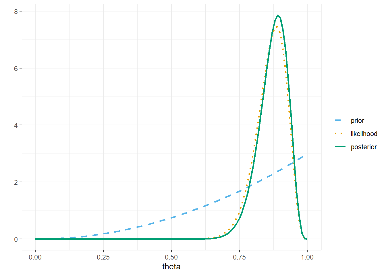
# 50% posterior credible interval
qbeta(c(0.25, 0.75), alpha_post, beta_post)
[1] 0.8398218 0.9105693# 80% posterior credible interval
qbeta(c(0.10, 0.90), alpha_post, beta_post)[1] 0.8005591 0.9345918# 98% posterior credible interval
qbeta(c(0.01, 0.99), alpha_post, beta_post)[1] 0.7239139 0.965060912.1.4 Prior predictive distribution
- Simulate \(\theta\) from the Beta(3, 1) prior distribution using
rbeta. - Given \(\theta\), simulate \(y\) from the Binomial(35, \(\theta\)) distribution.
- Simulate many \((\theta, y)\) pairs and summarize the simulated \(y\) values to approximate the prior predictive distribution.
n = 35

n_rep = 10000

# simulate theta from Beta prior distribution
theta_sim = rbeta(n_rep, alpha_prior, beta_prior)

# simulate y from Binomial(n, theta)
y_sim = rbinom(n_rep, n, theta_sim)

sim = data.frame(theta_sim, y_sim)

# display a few simulated pairs
sim |> head(10) |> kbl() |> kable_styling()| theta_sim | y_sim |
|---|---|
| 0.6280839 | 25 |
| 0.8274895 | 29 |
| 0.4882894 | 15 |
| 0.8900228 | 31 |
| 0.7641595 | 31 |
| 0.8126329 | 31 |
| 0.9561866 | 34 |
| 0.7012563 | 25 |
| 0.8672446 | 31 |
| 0.3422079 | 13 |
ggplot(data.frame(y_sim),
       aes(x = y_sim)) +
  geom_bar(aes(y = after_stat(prop)),
           col = bayes_col["posterior_predict"],
           fill = bayes_col["posterior_predict"],
           width = 0.1) +
  labs(x = "Number of successes",
       y = "Simulated relative frequency") +
  theme_bw()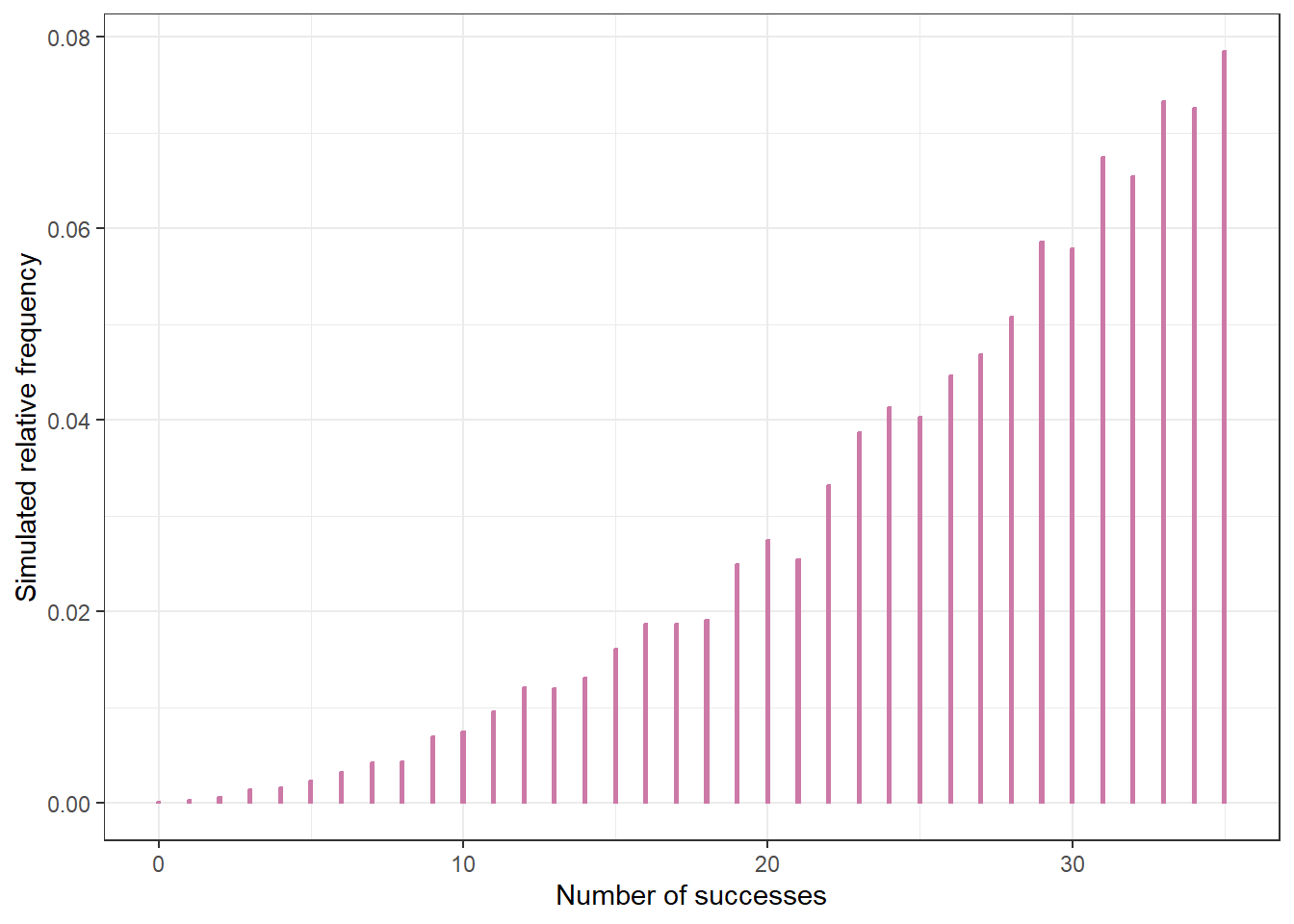
quantile(y_sim, 0.05)5%
12 12.1.5 Posterior predictive distribution
- Simulate \(\theta\) from the Beta(34, 5) posterior distribution using
rbeta. - Given \(\theta\), simulate \(y\) from the Binomial(35, \(\theta\)) distribution.
- Simulate many \((\theta, y)\) pairs and summarize the simulated \(y\) values to approximate the posterior predictive distribution.
n = 35

n_rep = 10000

# simulate theta from Beta posterior distribution
theta_sim = rbeta(n_rep, alpha_post, beta_post)

# simulate y from Binomial(n, theta)
y_sim = rbinom(n_rep, n, theta_sim)

sim = data.frame(theta_sim, y_sim)

# display a few simulated pairs
sim |> head(10) |> kbl() |> kable_styling()| theta_sim | y_sim |
|---|---|
| 0.8813914 | 29 |
| 0.9181022 | 33 |
| 0.8875739 | 30 |
| 0.8756327 | 30 |
| 0.9126112 | 30 |
| 0.7890674 | 27 |
| 0.6912154 | 24 |
| 0.8557116 | 30 |
| 0.8235766 | 30 |
| 0.8505959 | 29 |
ggplot(data.frame(y_sim),
       aes(x = y_sim)) +
  geom_bar(aes(y = after_stat(prop)),
           col = bayes_col["posterior_predict"],
           fill = bayes_col["posterior_predict"],
           width = 0.1) +
  labs(x = "Number of successes",
       y = "Simulated relative frequency") +
  theme_bw()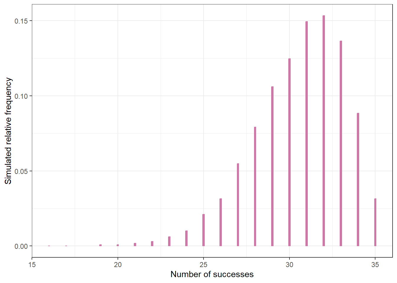
quantile(y_sim, c(0.025, 0.975)) 2.5% 97.5%
25 35 \(\theta\) is used to denote both: (1) the actual parameter (i.e., the random variable) \(\theta\) itself, and (2) possible values of \(\theta\).↩︎
When considering the prior predictive distribution \(y\) also denotes potential values of the data. For the posterior predictive distribution \(\tilde{y}\) denotes potential new values of the data.↩︎
The expression defines the shape of the Beta density. All that’s missing is the scaling constant which ensures that the total area under the density is 1. The actual Beta density formula, including the normalizing constant, is \[ p(u) =\frac{\Gamma(\alpha+\beta)}{\Gamma(\alpha)\Gamma(\beta)}\; u^{\alpha-1}(1-u)^{\beta-1}, \quad 0<u<1, \] where \(\Gamma(\alpha) = \int_0^\infty e^{-v}v^{\alpha-1} dv\) is the Gamma function. For a positive integer \(k\), \(\Gamma(k) = (k-1)!\). Also, \(\Gamma(1/2)=\sqrt{\pi}\).↩︎
When the prior and posterior distribution belong to the same family, that family is called a conjugate prior distribution for the likelihood. So, the Beta distributions form a conjugate prior family for Binomial distributions.↩︎