16  Normal-Normal Model

We have estimated the population mean of a Normal distribution, assuming known population standard deviation \(\sigma\), using grid approximation in Chapter 8 and posterior simulation in Section 14.1. We will relax the unreasonable assumption of known standard deviation soon. But before doing that, we will briefly investigate one more case where the posterior distribution can be derived analytically, in a form that makes explicit the relative influence of prior and likelihood.

Normal-Normal model¹

• Consider a measured variable \(y\) which, given \(\theta\), follows a Normal\((\theta, \sigma)\) distribution, with \(\sigma\) known.
• Suppose \(\theta\) has a Normal\((\mu_0, \tau_0)\) prior distribution.
• Let \(\bar{y}\) be the sample mean for a random sample of size \(n\).
• Then the posterior distribution of \(\theta\) given \(\bar{y}\) is the Normal\((\mu_n, \tau_n)\) distribution, where

\[\begin{align*} \text{posterior precision:} & &\frac{1}{\tau_n^2} & = \frac{1}{\tau_0^2} + \frac{n}{\sigma^2}\\ \text{posterior mean:} & & \mu_n & = \left(\frac{\frac{1}{\tau_0^2} }{\frac{1}{\tau_0^2} + \frac{n}{\sigma^2}}\right)\mu_0 + \left(\frac{\frac{n}{\sigma^2}}{ \frac{1}{\tau_0^2} + \frac{n}{\sigma^2}}\right)\bar{y}\\ \end{align*}\]

• The precision of a Normal distribution is the reciprocal of its variance.
• If \(y\) follows a Normal\((\theta, \sigma)\) distribution, the precision in a single measurement of \(y\) is \(1/\sigma^2\).
• For a random sample of \(n\) values of the variable \(y\), the sample mean \(\bar{y}\) follows a Normal distribution with standard deviation \(\sigma/\sqrt{n}\) and precision \(n/\sigma^2\). That is, the precision in \(n\) independent data values is \(n\) times the precision in a single value.
• For the posterior distribution in the Normal-Normal model, there is an intuitive interpretation of the compromise between prior and likelihood.
  • The posterior precision is the sum of the prior precision and the data precision.
  • The posterior mean is a weighted average of the prior mean and the sample mean, with weights proportional to the precisions.

	Prior	Data (Sample Mean)	Posterior
Precision	\(\frac{1}{\tau_0^2}\)	\(\frac{n}{\sigma^2}\)	\(\frac{1}{\tau_n^2} = \frac{1}{\tau_0^2}+\frac{n}{\sigma^2}\)
SD	\(\tau_0\)	\(\frac{\sigma}{\sqrt{n}}\)	\(\tau_n\)
Mean	\(\mu_0\)	\(\bar{y}\)	\(\mu_n = \left(\frac{\frac{1}{\tau_0^2} }{\frac{1}{\tau_0^2} + \frac{n}{\sigma^2}}\right)\mu_0 + \left(\frac{\frac{n}{\sigma^2}}{ \frac{1}{\tau_0^2} + \frac{n}{\sigma^2}}\right)\bar{y}\)

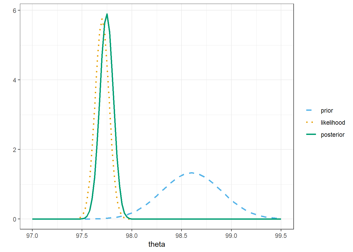
Example 16.1 Assume body temperatures (degrees Fahrenheit) of healthy adults follow a Normal distribution with unknown mean \(\theta\) and known standard deviation \(\sigma=1\). (It’s unrealistic to assume the population standard deviation is known. We’ll consider the case of unknown standard deviation later.) Suppose we wish to estimate \(\theta\), the population mean healthy human body temperature.
Assume the prior distribution of \(\theta\) is Normal with mean 98.6 and standard deviation 0.7.

The sample mean body temperature in a sample of 208 healthy adults is 97.7 degrees F.

1. Use the Normal-Normal model to identify the posterior distribution of \(\theta\). (Compare to the results of Chapter 8 and Section 14.1.)
   
   
   
   
   

2. Find a 98% posterior credible interval.
   
   
   
   
   

3. Considering each of the following changes in isolation, indicate if (1) the center and (2) the width of the posterior credible interval would be greater than, less than, or equal to the respective values from the previous part.

   1. Credibility is 80%
      
      
      
      
      

   2. Sample size is 20
      
      
      
      
      

   3. Sample mean is 98.0
      
      
      
      
      

   4. Prior mean is 98.0
      
      
      
      
      

   5. Prior SD is 0.1
      
      
      
      
      

   6. Population SD is \(\sigma = 0.5\)
      
      
      
      
      

16.1 Notes

The code below just plugs the numbers into the above Normal-Normal model formulas.

# prior
mu0 = 98.6
tau0 = 0.3

# data
sigma = 1
n = 208
ybar = 97.7

# posterior
tau_n = 1 / sqrt(n / sigma ^ 2 + 1 / tau0 ^ 2)
mu_n = mu0 * (1 / tau0 ^ 2) / (1 / tau_n ^ 2) + ybar * (n / sigma ^ 2) / (1 / tau_n ^ 2)

df = data.frame(c("Precision", "SD", "Mean"),
                c(1 / tau0 ^ 2, tau0, mu0),
                c(n / sigma ^ 2, sigma / sqrt(n), ybar),
                c(1 / tau_n ^ 2, tau_n, mu_n))

df |>
  kbl(digits = 3,
      col.names = c("", "Prior", "Data (Sample Mean)", "Posterior")) |>
  kable_styling()

	Prior	Data (Sample Mean)	Posterior
Precision	11.111	208.000	219.111
SD	0.300	0.069	0.068
Mean	98.600	97.700	97.746

# scaled likelihood, depends on data: n, ybar
likelihood_scaled <- function(theta) {
  likelihood <- function(theta) {
    dnorm(x = ybar, mean = theta, sd = sigma / sqrt(n))
  }
  scaling_constant <- integrate(likelihood, lower = 95, upper = 100)[[1]]
  likelihood(theta) / scaling_constant
}

# Plot
ggplot(data.frame(x = c(97.0, 99.5)),
       aes(x = x)) +
  # prior
  stat_function(fun = dnorm,
                args = list(mean = mu0,
                            sd = tau0),
                lty = bayes_lty["prior"],
                linewidth = 1,
                aes(color = "prior", linetype = "prior")) +
  # (scaled) likelihood
  stat_function(fun = likelihood_scaled,
                lty = bayes_lty["likelihood"],
                linewidth = 1,
                aes(color = "likelihood", linetype = "likeihood")) +
  # posterior
  stat_function(fun = dnorm,
                args = list(mean = mu_n,
                            sd = tau_n),
                lty = bayes_lty["posterior"],
                linewidth = 1,
                aes(color = "posterior", linetype = "posterior")) +
  # Define color and add a legend
  scale_color_manual(name = "",
                     breaks = c("prior", "likelihood", "posterior"),
                     values = bayes_col[c("prior", "likelihood", "posterior")]) +
  scale_linetype_manual(name = "",
                        breaks = c("prior", "likelihood", "posterior"),
                        values = bayes_lty[c("prior", "likelihood", "posterior")]) +
  labs(x = "theta",
       y = "") +
  theme_bw()

Warning: No shared levels found between `names(values)` of the manual scale and the
data's linetype values.

qnorm(c(0.01, 0.10, 0.25, 0.75, 0.90, 0.99), mu_n, tau_n)

[1] 97.58848 97.65906 97.70007 97.79121 97.83222 97.90280

---

1. Try this applet which illustrates the Normal-Normal model.