29  Stochastic Processes

Example 29.1 Select a U.S. city at random. For each of the following suggest what an output would look like.

1. Record the current temperature in the city.
   
   
   
   
   

2. Record the current temperature and today’s high temperature in the city.
   
   
   
   
   

3. Record the daily high temperature in the city each day for the next month.
   
   
   
   
   

4. Record the temperature in the city continuously for the next 24 hours.
   
   
   
   
   

• A random variable assigns a number to each outcome of a random phenomenon.
  • A random variable is a function \(X\) that takes an outcome in the sample space for the random phenomenon as input and returns a real number as output.
  • There are often multiple random variables defined on the same probability space. For two random variables \(X\) and \(Y\), each outcome will generate an \((x,y)\) pair of values.
• A stochastic process (a.k.a. random¹ process) is an indexed collection of random variables (which are usually dependent): \(\{X(t): t\in T\}\) where \(T\) is some index set.
  • \(t\) is usually interpreted as “time”, so \(X(t)\) (also denoted \(X_t\)) represents the value at time \(t\) for some random process which occurs over time.
  • When the time index set is countable, e.g. \(T=\{0, 1, 2, \ldots\}\), the collection \(\{X_0, X_1, X_2, \ldots\}\) is called a discrete time stochastic process.
  • When the time index set is uncountable, e.g. \(T=[0,\infty)\), the collection \(\{X(t), t\ge0\}\) is called a continuous time stochastic process.
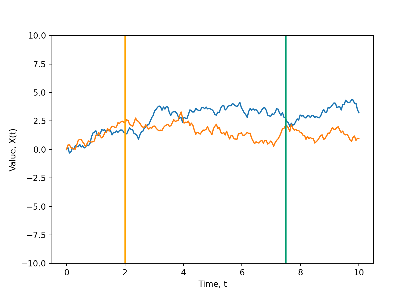
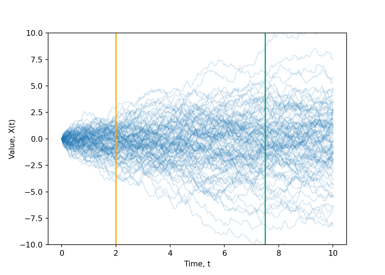
• For a given outcome in the sample space of the random phenomenon, a stochastic process \(\{X(t)\}\) outputs a sample path (a.k.a. sample function) which describes how the value of the process evolves over time for that particular outcome.
  • A random variable \(X\) maps outcomes of the random phenomenon to real numbers.
  • A continuous time stochastic process \(\{X(t), t\ge 0\}\) maps outcomes of the random phenomenon to functions (of \(t\)).
  • A discrete time stochastic process \(\{X_0, X_1, X_2, \ldots\}\) maps outcomes of the random phenomenon to sequences.
• The set of all possible sample paths for the random phenomenon is called the ensemble of the stochastic process.
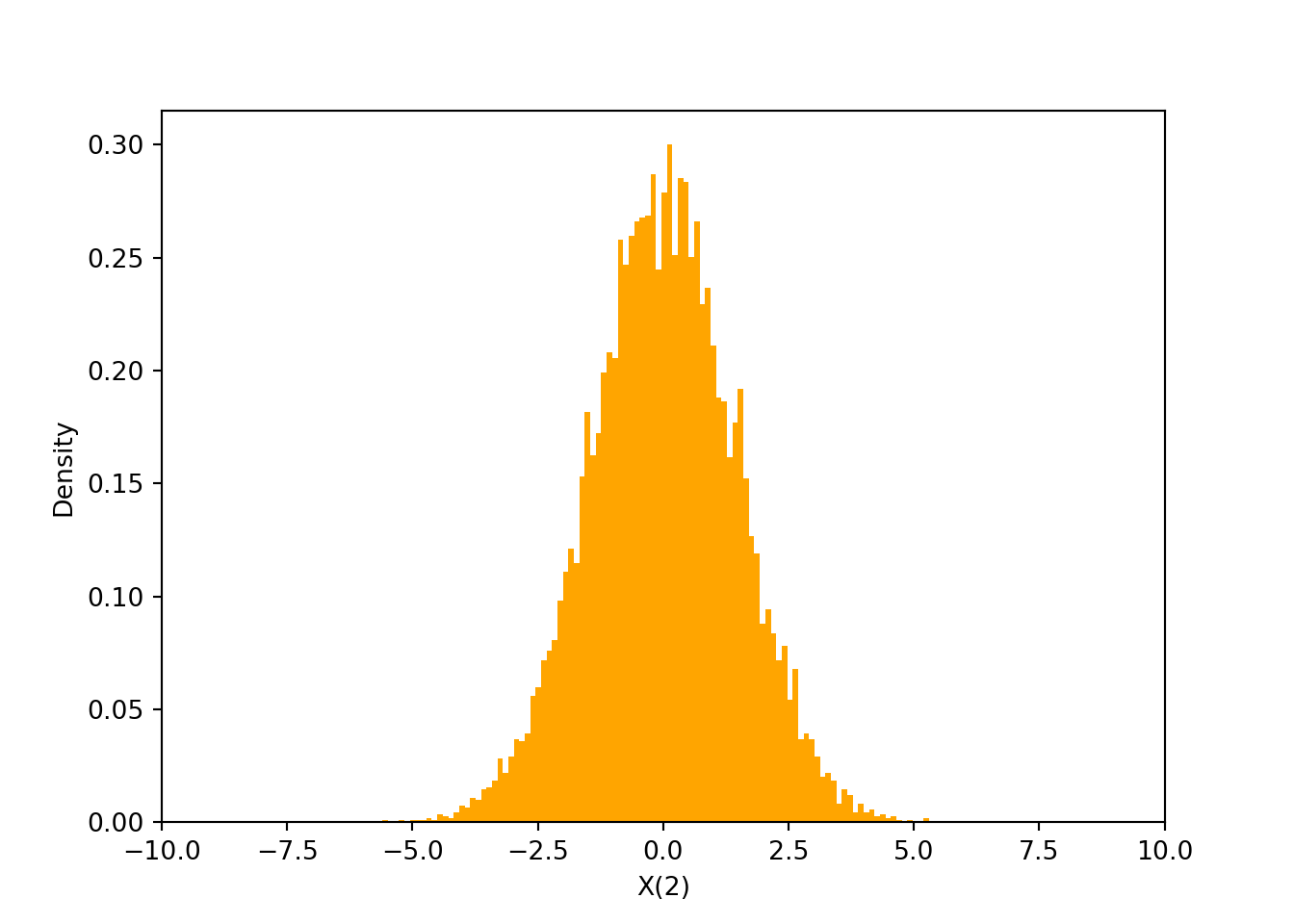
• Essential concept: At each fixed point in time \(t\), \(X(t)\) is a random variable, and so it has a (marginal) distribution.
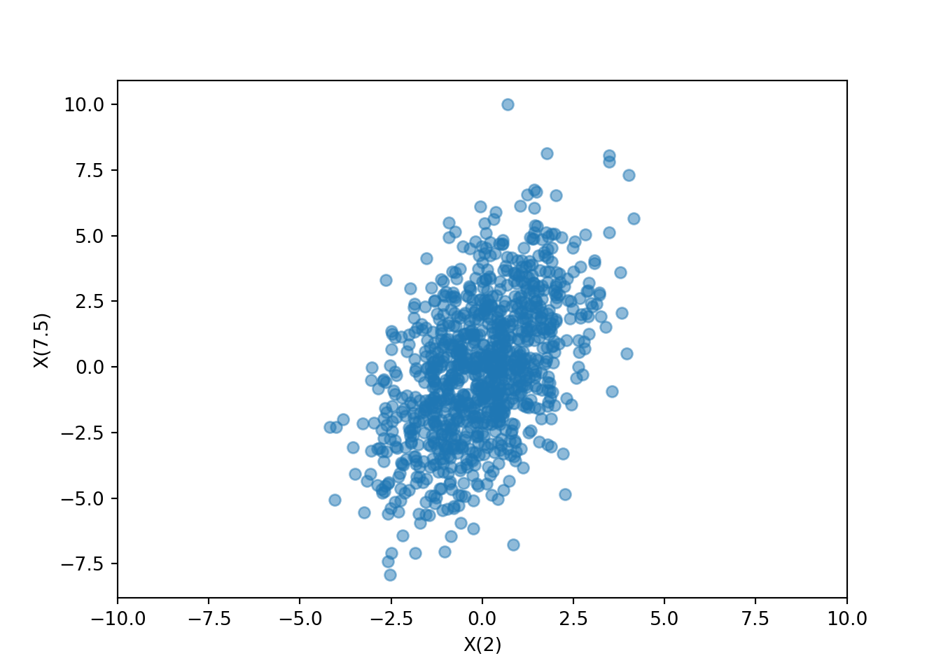
  • The process values \(X(t)\) and \(X(s)\) at any two points in time, \(s\) and \(t\), have a joint distribution.
• If for all times the process takes values in some set \(S\), then \(S\) is called the state space of the stochastic process.
  • If \(S\) is a countable set, then the process is a discrete state process.
  • If \(S\) is an uncountable set, then the process is a continuous state process.
• There is a single state space for the entire process. (That is, there is NOT a different state space for each point in time.)
  • Whether the process is discrete-state or continuous-state depends on the state space, which depends on how the process behaves over all times (and not what happens at any particular time)
• There are two main perspectives from which we consider stochastic processes
  • Sample path: Fix an outcome and view the process values over all times
  • Random variable: Fix a time and view the process values over all outcomes

(a) Two sample paths

(b) Many sample paths

Figure 29.1: Sample paths of a stochastic process X(t), with times t=2 and t=7.5 highlighted

(a) Marginal distribution of X(7.5), process value at time t=7.5

(b) Joint distribution of X(2) and X(7.5), process values at times t=2 and t=7.5

(c) Marginal distribution of X(2), process value at time t=2

Figure 29.2: Distributions associated with the process in Figure 29.1

Example 29.2 Harry and Tom play a game which involves flipping a fair coin. Each time the coin lands on heads, Tom pays Harry 1 dollar; each time the coin lands on tails, Harry pays Tom 1 dollar. Let \(X_n\) denote Harry’s cumulative winnings after \(n\) flips, with \(X_0=0\), and with negative values denoting losses.

1. Simulate and sketch a single sample path (for \(n=0,1,2,3,4\)).
   
   
   
   
   

2. Is the \(\{X_n\}\) process discrete- or continuous- time? Discrete- or continuous- state? Assuming they keep playing the game forever, what is the state space?
   
   
   
   
   

3. Find the distribution of \(X_2\).
   
   
   
   
   

4. Find the joint distribution of \(X_2\) and \(X_3\).
   
   
   
   
   

Example 29.3 An intended signal may have the form \(a \cos(2\pi t)\), but amplitude variation may occur (due to natural current or voltage variation). Consider the stochastic process \[ X(t) = A \cos(2\pi t) \] where \(A\) is a random variable whose distribution describes the amplitude variation.

1. Suppose that \(A\) is equally likely to be 0.5, 1, or 2. Sketch the ensemble of this stochastic process.
   
   
   
   
   

2. Is the \(\{X(t)\}\) process discrete- or continuous- time? Discrete- or continuous- state? What is the state space?
   
   
   
   
   

3. Find the distribution of \(X(1)\).
   
   
   
   
   

4. Find the distribution of \(X(2/3)\).
   
   
   
   
   

5. Find the distribution of \(X(0.25)\).
   
   
   
   
   

6. Suppose that \(A\) has an Exponential(1) distribution. Sketch some sample paths of the \(\{X(t)\}\) process.
   
   
   
   
   

7. Find the distribution of \(X(1)\).
   
   
   
   
   

8. Find the distribution of \(X(2/3)\).
   
   
   
   
   

9. Find the distribution of \(X(0.25)\).
   
   
   
   
   

Example 29.4 A deterministic signal \(s(t)\) may incur “additive noise” during transmission, in which case the received message has the form \(X(t) = s(t) + N(t)\). Supposed that the received signal is \[ X(t) = 3\cos(2\pi t) + N(t), \] where, \(N(t)\) is a “Gaussian white noise process”, for which at any time \(t\), \(N(t)\) has a Normal (Gaussian) distribution with mean 0 and standard deviation 1.

1. Find the distribution of \(X(1)\).
   
   
   
   
   

2. Find the distribution of \(X(0.25)\).
   
   
   
   
   

---

1. The words stochastic and random are synonynms; stochastic is Greek in origin, while random is French. The notation \(X(t)\) is often used to denote both the process as a whole, and the value of the process at time \(t\). It is usually clear from context which it is. Sometimes the process is written as \(\{X(t)\}\) to emphasize the distinction.