5  Introduction to Simulation

• Simulation involves using a probability model to artificially recreate a random phenomenon, many times, usually using a computer.
• Given a probability model, we can simulate outcomes, occurrences of events, and values of random variables, according to the specifications of the probability measure which reflects the model assumptions.
• In general, a simulation involves the following steps.
  1. Set up. Define a probability space, and related random variables and events.
  2. Simulate. Simulate — according to the assumptions reflected in the probability measure — outcomes, occurrences of events, and values of random variables.
  3. Summarize. Summarize simulation output in plots and summary statistics (relative frequencies, averages, standard deviations, correlations, etc) to describe and approximate probabilities, distributions, and related characteristics.
  4. Sensitivity analysis. Investigate how results respond to changes in the assumptions or parameters of the simulation.
• Many random phenomena can be concretely represented in terms of “box models” and “spinners”.

Example 5.1 Let \(X\) be the sum of two rolls of a fair four-sided die, and let \(Y\) be the larger of the two rolls (or the common value if a tie).

1. Set up a “box model” and explain how you would use it to simulate a single realization of the pair \((X, Y)\). Could you use a spinner instead?
   
   
   
   
   

2. Suppose the die is weighted so that is lands on 1 with probability 0.1, 2 with probability 0.2, 3 with probability 0.3, and 4 with probability 0.4. Describe a box model and a spinner to represent this weighted die.
   
   
   
   
   

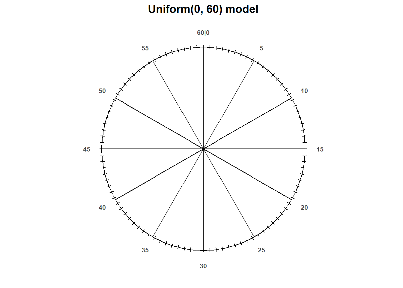
Example 5.2 Recall the meeting problem where Regina and Cady will definitely arrive between noon and 1:00, but their exact arrival times are uncertain. Rather than dealing with clock time, it is helpful to represent noon as time 0 and measure time as minutes after noon, so that arrival times take values in the continuous interval [0, 60].

1. Suppose they are “equally likely” to arrive at any time between noon and 1:00, independently of each other. Explain how you would construct a spinner and use it to simulate an outcome.
   
   
   
   
   

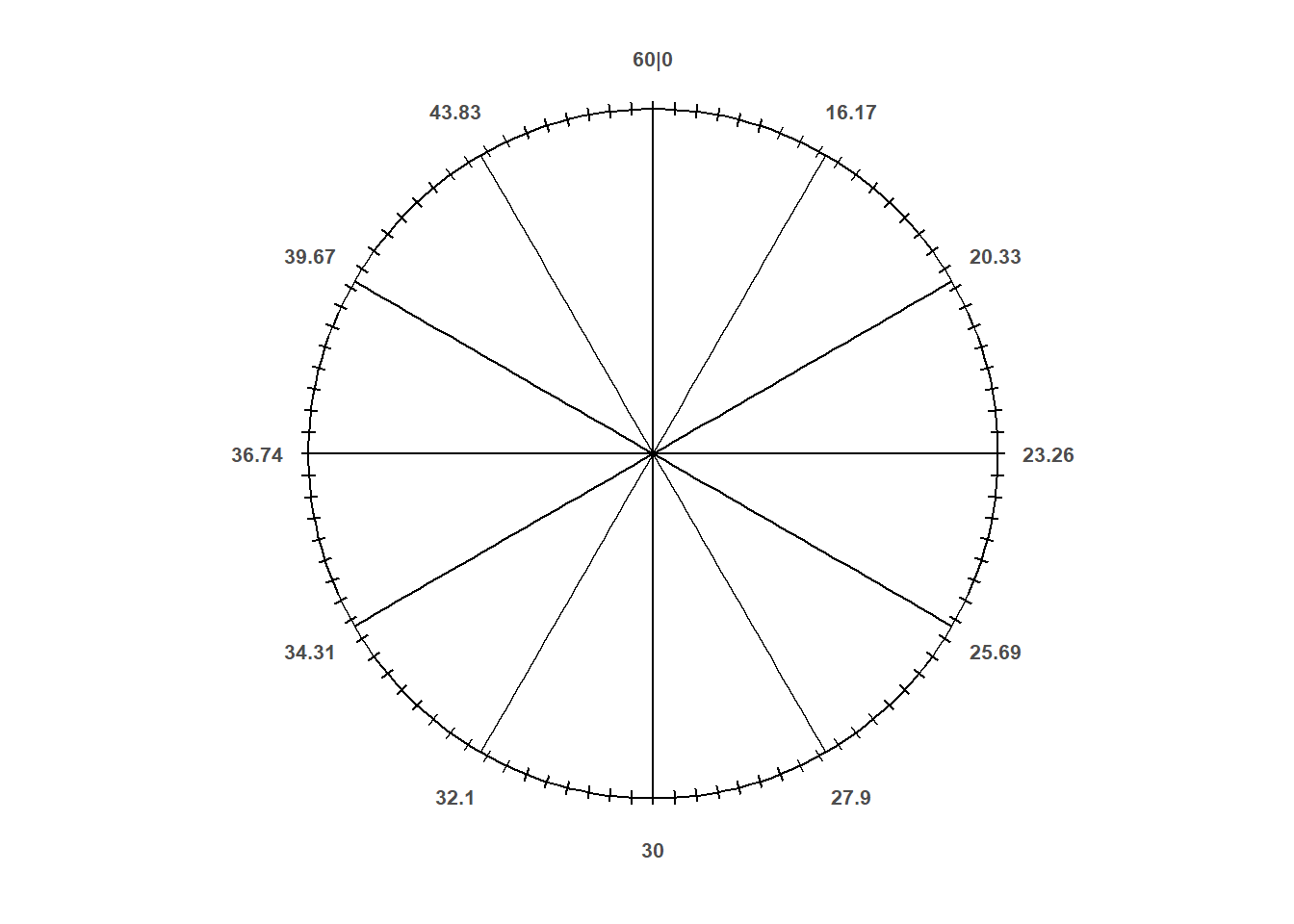
2. Suppose they are more likely to arrive near 12:30 and less likely to arrive near 12:00 or 1:00, independently of each other. How could you construct a circular spinner to represent these assumptions? Imagine the spinner needle is still equally likely to point at any value on the circular axis.
   
   
   
   
   

• The probability of event \(A\) can be approximated by simulating, according to the assumptions corresponding to the probability measure \(\text{P}\), the random phenomenon a large number of times and computing the relative frequency of \(A\).

\[ {\small \text{P}(A) \approx \frac{\text{number of repetitions on which $A$ occurs}}{\text{number of repetitions}}, \quad \text{for a large number of $\text{P}$-repetitions} } \]

Example 5.3 Use a fair four-sided die (or a box or a spinner) and perform by hand 10 repetitions of the simulation in Example 5.1. For each repetition, record the results of the first and second rolls (or draws or spins) and the values of \(X\) and \(Y\). Based only on the results of your simulation, how would you approximate the following? (Don’t worry if the approximations are any good yet.)

1. \(\text{P}(A)\), where \(A\) is the event that the first roll is 3.
   
   
   
   
   
2. \(\text{P}(X=6)\)
   
   
   
   
   
3. \(\text{P}(Y = 3)\)
   
   
   
   
   
4. \(\text{P}(X=6, Y=3)\)
   
   
   
   
   
5. Will the results above tend to produce good estimates of the corresponding theoretical values? Why? If not, how could we improve the estimates?
   
   
   
   
   

• In practice, many repetitions of a simulation are performed on a computer to approximate what happens in the “long run”.
• However, we often start by carrying out a few repetitions, (1) by hand to help make the process more concrete, or (2) by computer to check that our code is working correctly

Example 5.4 Recall the meeting problem. Describe in detail how, in principle, you could conduct by hand a simulation and use the results to approximate the probability that Regina and Cady arrive with 15 minutes of each other for the following two models.

1. Uniform(0, 60), independent arrivals model

Figure 5.1: Uniform(0, 60) spinner

2. Normal(30, 10), independent arrivals model

Figure 5.2: Normal(30, 10) spinner

• A probability is a theoretical long run relative frequency.
• A probability can be approximated by a relative frequency from a large number of simulated repetitions, but there is some simulation margin of error, due to natural variability in the simulation.
• The margin of error when approximating a single probability based on a simulated relative frequency is roughly on the order \(1/\sqrt{N}\), where \(N\) is the number of independently simulated values used to calculate the relative frequency.
• Use a margin of error of \(2/\sqrt{N}\) when simultaneously approximating many probabilities based on a single simulation.